
Urban Water Quality Prediction Based on Multi-Task Multi-View Learning
Proceedings of the Twenty-Fifth International Joint Conference on Artificial Intelligence. Pages 2576-2580.
© 2016 International Joint Conferences on Artificial Intelligence
Abstract
Urban water quality is of great importance to our daily lives. Prediction of urban water quality help control water pollution and protect human health. In this work, we forecast the water quality of a station over the next few hours, using a multi-task multi-view learning method to fuse multiple datasets from different domains. In particular, our learning model comprises two alignments. The first alignment is the spaio-temporal view alignment, which combines local spatial and temporal information of each station. The second alignment is the prediction alignment among stations, which captures their spatial correlations and performs co-predictions by incorporating these correlations. Extensive experiments on real-world datasets demonstrate the effectiveness of our approach.
- [Beck and Teboulle, 2009] Amir Beck and Marc Teboulle. A fast it- erative shrinkage-thresholding algorithm for linear inverse prob- lems. SIAM Journal on Imaging Sciences, 2(1):183-202, 2009.
- [Castro and Neves, 2003] Pedro Castro and Mário Neves. Chlo- rine decay in water distribution systems case study-lousada net- work. Electronic Journal of Environmental, Agricultural and Food Chemistry, 2(2):261-266, 2003.
- [Evgeniou and Pontil, 2004] Theodoros Evgeniou and Massimil- iano Pontil. Regularized multi-task learning. In Proceedings of the ACM SIGKDD international conference on Knowledge dis- covery and data mining, pages 109-117, 2004.
- [He and Lawrence, 2011] Jingrui He and Rick Lawrence. A graph- based framework for multi-task multi-view learning. In Proceed- ings of the International Conference on Machine Learning, pages 25-32, 2011.
- [Lin et al., 2003] Jessica Lin, Eamonn Keogh, Stefano Lonardi, and Bill Chiu. A symbolic representation of time series, with implica- tions for streaming algorithms. In Proceedings of the ACM SIG- MOD Workshop on Research Issues in Data Mining and Knowl- edge Discovery, pages 2-11, 2003.
- [Liu et al., 2015] Ye Liu, Liqiang Nie, Lei Han, Luming Zhang, and David S. Rosenblum. Action2activity: Recognizing com- plex activities from sensor data. In Proceedings of the Interna- tional Joint Conference on Artificial Intelligence, pages 1617- 1623, 2015. IJCAI
- [Liu et al., 2016a] Ye Liu, Liqiang Nie, Li Liu, and David S. Rosen- blum. From action to activity: Sensor-based activity recognition. Neurocomputing, 181:108-115, 2016.
- [Liu et al., 2016b] Ye Liu, Luming Zhang, Liqiang Nie, Yan Yan, and David S Rosenblum. Fortune teller: Predicting your career path. In Proceedings of the AAAI Conference on Artificial Intel- ligence, 2016.
- [Luo et al., 2015] Ge Luo, Ke Yi, Siu-Wing Cheng, Zhenguo Li, Wei Fan, Cheng He, and Yadong Mu. Piecewise linear approxi- mation of streaming time series data with max-error guarantees. In Proceedings of the IEEE International Conference on Data Engineering, pages 173-184, 2015.
- [Monteiro et al., 2014] L Monteiro, D Figueiredo, S Dias, R Fre- itas, D Covas, J Menaia, and ST Coelho. Modeling of chlorine decay in drinking water supply systems using epanet msx. Pro- cedia Engineering, 70:1192-1200, 2014.
- [Nesterov, 2013] Yurii Nesterov. Introductory lectures on convex optimization: A basic course, volume 87. 2013.
- [Organization, 2004] World Health Organization. Guidelines for drinking-water quality, volume 3. 2004.
- [Rossman and Boulos, 1996] Lewis A Rossman and Paul F Boulos. Numerical methods for modeling water quality in distribution systems: A comparison. Journal of Water Resources planning and management, 122(2):137-146, 1996.
- [Rossman et al., 1994] Lewis A Rossman, Robert M Clark, and Walter M Grayman. Modeling chlorine residuals in drinking- water distribution systems. Journal of environmental engineer- ing, 120(4):803-820, 1994.
- [Tibshirani, 1996] Robert Tibshirani. Regression shrinkage and se- lection via the lasso. Journal of the Royal Statistical Society. Series B (Methodological), pages 267-288, 1996.
- [Tobler, 1970] Waldo R Tobler. A computer movie simulating ur- ban growth in the detroit region. Economic geography, pages 234-240, 1970.
- [Wang et al., 2014] Yilun Wang, Yu Zheng, and Yexiang Xue. Travel time estimation of a path using sparse trajectories. In Proceedings of the ACM SIGKDD international conference on Knowledge discovery and data mining, pages 25-34, 2014.
- [Xue et al., 2013] Andy Yuan Xue, Rui Zhang, Yu Zheng, Xing Xie, Jin Huang, and Zhenghua Xu. Destination prediction by sub-trajectory synthesis and privacy protection against such pre- diction. In Proceedings of the IEEE International Conference on Data Engineering, pages 254-265, 2013.
- [Yuan and Lin, 2006] Ming Yuan and Yi Lin. Model selection and estimation in regression with grouped variables. Journal of the Royal Statistical Society: Series B (Statistical Methodology), 68(1):49-67, 2006.
- [Zhang and Huan, 2012] Jintao Zhang and Jun Huan. Inductive multi-task learning with multiple view data. In Proceedings of the ACM International Conference on Knowledge Discovery and Data Mining, pages 543-551, 2012.
- [Zhang et al., 2013] Wei Zhang, Ke Zhang, Pan Gu, and Xiangyang Xue. Multi-view embedding learning for incompletely labeled data. In Proceedings of the International Joint Conference on Artificial Intelligence, pages 1910-1916, 2013. IJCAI
- [Zhao et al., 2015] Liang Zhao, Qian Sun, Jieping Ye, Feng Chen, Chang-Tien Lu, and Naren Ramakrishnan. Multi-task learn- ing for spatio-temporal event forecasting. In Proceedings of the ACM International Conference on Knowledge Discovery and Data Mining, pages 1503-1512, 2015.
- [Zheng et al., 2014] Yu Zheng, Licia Capra, Ouri Wolfson, and Hai Yang. Urban computing: Concepts, methodologies, and applica- tions. ACM Transactions on Intelligent Systems and Technology, 5(3):38:1-38:55, 2014.
- [Zheng et al., 2015a] Yu Zheng, Xiuwen Yi, Ming Li, Ruiyuan Li, Zhangqing Shan, Eric Chang, and Tianrui Li. Forecasting fine- grained air quality based on big data. In Proceedings of the ACM SIGKDD International Conference on Knowledge Discovery and Data Mining, pages 2267-2276, 2015.
- [Zheng et al., 2015b] Yu Zheng, Huichu Zhang, and Yong Yu. Detecting collective anomalies from multiple spatio-temporal datasets across different domains. In Proceedings of the SIGSPA- TIAL International Conference on Advances in Geographic In- formation Systems, pages 1-10, 2015.
- [Zheng, 2015] Yu Zheng. Methodologies for cross-domain data fu- sion: An overview. IEEE Transactions on Big Data, 1(1):16-34, 2015.
- [Zhou et al., 2011] Jiayu Zhou, Jianhui Chen, and Jieping Ye. Mal- sar: Multi-task learning via structural regularization. Arizona State University, 2011.
References were extracted automatically from the PDF and may contain errors.
Full text extracted automatically from the PDF; figures, tables and equations may differ. The PDF is the version of record.
1 Introduction
Urban water is a vital resource that affects various aspects of human, health and urban lives. Urban water quality, which serves as "a powerful environmental determinant" and "a foundation for the prevention and control of waterborne diseases" [Organization, 2004], refers to the physical, chemical and biological characteristics of a water body, and several chemical indexes (such as residual chlorine, turbidity and pH) can be used as effective measurements for the water quality in current urban water distribution systems [Rossman et al., 1994]. With the increasing demand for water quality information, several water quality monitoring stations have been deployed throughout the city's water distribution system to provide the real-time water quality reports in a city. Besides water quality monitoring, predicting the urban water quality plays an essential role in many urban aquatic projects, such as informing waterworks' decision making (e.g., pre-adjustment of chlorine from the waterworks), affecting governments' policy making (e.g., issuing pollution alerts or performing a pollution control), and providing maintenance suggestions (e.g., suggestions for replacements of certain pipelines).
⇤The paper was done when the first and third authors were interns in Microsoft Research under the supervision of the second author. Yu Zheng is the correspondence author of this paper.
However, predicting urban water quality is very challenging due to the following reasons. First, the water quality of a station is affected by multiple complex factors, including spatial factors (e.g., pipe attributes) and temporal factors (e.g., flow and pressure). Capturing these complex factors as well as the spatio-temporal heterogeneity simultaneously is a tough challenge. Existing hydraulic models-based approaches try to model water quality from physical and chemical perspective, but such hydraulic models can hardly capture all of those complex factors. Moreover, the parameters in models are hard to get, which makes it difficult to extend to other water distribution systems. Second, as all the stations are connected through the pipeline system, the water quality among different stations are mutually correlated by several complex factors, such as attributes in pipe networks and distribution of Points of Interests (POIs). Therefore, characterizing such relatedness globally is another challenge. Traditional hydraulic models-based approaches build hydraulic models for each station and ignore their spatial correlations, and thus their performance is far from satisfactory.
To address the aforementioned issues, in this paper, we predict the water quality of a station through a data-driven perspective using a variety of data sets, including water quality data, hydraulic data, meteorology data, pipeline networks data, road networks data, and POIs. In particular, we present a novel spatio-temporal multi-task multi-view learning (stMTMV) framework to fuse the heterogeneous data from multiple domains and jointly capture each station's local information as well as their global information. It coregularizes the following factors: (1) Spatio-temporal View Alignment. The water quality of each station is characterized by a spatial view and a temporal view. Since both views describe the water quality of a station, their prediction results should be similar. Thus, the view alignment is employed to penalize their disagreements. (2) Global Prediction Alignment. The prediction of water quality at each station is a treated as a task. As all the stations are connected via the pipe network, two stations that are near tend to have similar readings compared to two stations that are far. Therefore, a graph Laplacian regularizer is introduced to capture the spatial correlation among tasks, which is also consistent with Toblers first law of geography [Tobler, 1970]. (3) Feature Learning. Features extracted from spatial and temporal views are usually in high-dimension spaces. We employ a group Lasso [Yuan and Lin, 2006] to identify the discriminant taskspecific and task-sharing features automatically.
We summarize the contributions as follows:
- ÷ We present a novel data-driven approach to co-predict the future water quality among different stations with data frommultiple domains. Additionally, the approach is not restricted to urban water quality prediction, but also can be applied to other multi-locations based coprediction problem in many other urban applications.
- ÷ We present a novel spatio-temporal multi-view multitask learning framework (stMTMV) to integrate multiple sources of spatio-temporal urban data, which provides a general framework of combining heterogeneous spatio-temporal properties for prediction, and can also be applied to other spatio-temporal based applications.
2 Framework Overview
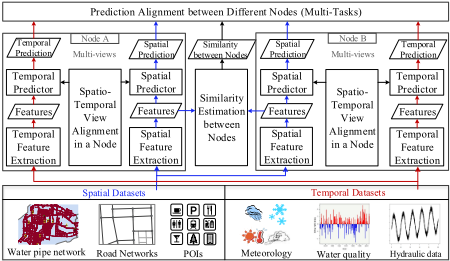
Figure 1 presents the framework of our approach, consisting of two major components. One is local spatio-temporal view alignment within a station (node), and the other is global prediction alignment among stations (nodes). In particular, after constructing the spatial and temporal views by extracting spatial- and temporal-related features for each station from spatial datasets (e.g., water pipe network, POIs) and temporal datasets (e.g., water quality data, hydraulic data), we predict the water quality from each station's local information by combining its spatial and temporal views. Meanwhile, as the water quality among stations are mutually correlated through the complex water distribution system, we thus can co-predict the water quality over all stations by capturing their spatial correlations, which is encoded by the structure of water distribution system.
3 Data Analysis
Urban water quality refers to the physical, chemical and biological characteristics of a water body [Rossman et al., 1994].
In current urban water distribution systems, three important quality indexes, i.e., residual chlorine, turbidity and pH, are used as effective measurements for the water quality [Organization, 2004]. In this paper, we consider Residual Chlorine (RC) as the water quality index since it is widely employed as the major quality index in environmental science [Organization, 2004; Rossman et al., 1994].
The concentration of RC is influenced by multiple temporal factors, such as turbidity, pH, flow, pressure and meteorology [Rossman et al., 1994; Monteiro et al., 2014]. For instance, turbidity normally exhibits opposite trend with RC since the chemical reactions of RC with pipe and bulk fluid will consume RC and increase the turbidity in water [Castro and Neves, 2003], where this negative correlation can also be observed from data as shown in Figure 2(a). As another example, water flow is also closely related to water quality, which has been identified in the environmental research [Rossman and Boulos, 1996; Castro and Neves, 2003]. The reason is that flow affects the time that water stays in the system and longer stay will result in a higher consumption of RC when compared to shorter stay.
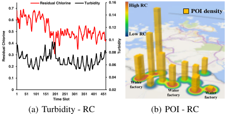
Besides temporal factors, the water quality also depends on several spatial factors, such as pipe network structures, POIs, road networks [Rossman and Boulos, 1996; Castro and Neves, 2003]. For example, the categories of POIs and their distributions in a region indicate the functionality as well as the water usage patterns in that region, therefore affecting the water quality of that region. Figure 2(b) depicts the correlation between POI density and RC from data, where each pillar denotes a station and the height of a pillar means the POI density around a station. From this figure, it can be seen that a high density of POIs can cause the concentration of RC to be high in that region. Similarly, the attributes of pipe network, such as length, diameter and age, are also factors that influence the water quality.
4 Spatio-temporal Views Construction
4.1 Temporal View
The temporal view of a station is constructed by incorporating its local temporal information, which consists of historical water quality indexes, historical hydraulic characteristics and meteorological information. In particular, we use the latest 12 hours temporal data in a station, such as water quality data (RC, Turbidity, pH) and water hydraulic data (flow, pressure), and treated them as time series signals. To capture the characteristics of the signal comprehensively, we extract statistical features (mean, variance, maximum, minimum, skewness and kurtosis), and time series features (autocorrelation, PAA [Lin et al., 2003], PLA [Luo et al., 2015]) for each of the time series above. Moreover, we also extract frequency related features (FFT and DWT) for each time series, where we only use the top 3 coefficients and discard others. In addition, we employ temperature, humidity, barometer pressure, wind speed, and weather as the meteorological features. The temporal view is constructed by concatenating all the temporal features above into a single feature vector.
4.2 Spatial View
The spatial view of a station is built by integrating its local spatial information, comprising pipe network structures, road network structures and distribution of POIs. In particular, for a given station, we extract the pipe attribute features (length, diameter and age), POI features (distribution of POIs), road network features (road segment density, road length). Moreover, the water quality of a station is also affected by its neighbors since RC are dispersed through the water distribution system. The impact of other stations on a particular station depends on multiple complex spatial factors, such as their connectivity in the pipe network and their geographical similarity. To encode such effects, we consider the water quality and hydraulic characteristics from a station's neighborhood, which can also capture the spatial information of a station. More specifically, we find k nearest neighbors for a given station and aggregate its neighbors' temporal features via the geographical similarity, where the geographical similarity is computed by the sum of top-k shortest paths between two stations. Therefore, the spatial view is constructed by concatenating all the spatial features as well as the aggregated surrounding temporal features into a single feature vector.
5 UrbanWater Quality Prediction
5.1 Notations
We first define some notations. In particular, we use bold capital letters (e.g., X) and bold lowercase letters (e.g., x) to denote matrices and vectors, respectively. We employ nonbold letters (e.g., x) to represent scalars, and Greek letters (e.g., λ) as parameters. Unless stated, otherwise, all vectors are in column form.
Let us assume that we have M nodes for the water quality prediction and each node is aligned with a task. Meanwhile, each node l is described by its spatial view Xsl 2 RNl⇥Ds = [xsl↪1 ↪ xsl↪2 ↪ ▷ ▷ ▷ ↪ xsl↪Nl ]T and temporal view Xtl 2 RNl⇥Dt = [xtl↪1 ↪ xtl↪2 ↪ ▷ ▷ ▷ ↪ xtl↪Nl ]T , where xsl↪i 2 RDs and xtl↪i 2 RDt denote the spatial feature and temporal feature extracted from the node l at time point i. Nl is the number of samples at node l, and Ds and Dt is the feature dimension of the spatial view and temporal view, respectively. The whole feature matrix at node l can be written as Xl = [Xsl ↪ Xtl ] 2 RNl⇥D , where D = Ds+Dt. The target vector at node l is denoted as yl = ¶yl↪1↪ yl↪2↪ ▷ ▷ ▷ ↪ yl↪Nl ♦ 2 RNl , which represents the water quality of node l observed at the discrete time points
1↪ 2↪ ▷ ▷ ▷ ↪Nl. N = PMl=1 Nl is the total number of samples over all tasks.
5.2 ProblemFormulation
The prediction at each node l consists of spatial prediction and temporal prediction, i.e., f s l (Xsl ) = Xsl wsl for spatial prediction and f t l (Xtl ) = Xtl wtl for temporal prediction, where wsl 2 RDs and wtl 2 RDt denote the linear mapping function for the task (node) l with spatial view and temporal view, respectively. In this paper, linear function is employed for simplicity. However, the model can be easily extended to other convex, smooth and non-linear prediction functions. Without prior knowledge on the contributions of spatial and temporal view, we assume that both contribute equally. Thus, the final prediction model of both spatial and temporal view for task (node) l is obtained by the following late fusion:
where wl 2 RD is the weight vector for task l. The weight matrix over M tasks (nodes) is denoted as W = [w1↪ w2↪ ▷ ▷ ▷ ↪ wM] 2 RD⇥M .
Information distributed in spatial and temporal views in fact describes the inherent characteristics of the same node from various aspects, we thus can reinforce the learning performance of individual views by enforcing the agreement on the their prediction results. Considering the least-squares loss function, we can define the following objective function:
In a real pipeline system, each node is not only affected by its local information, but also affected by the information from its neighbors or other nodes. To consider the global impact on node l, we expand the model in Eqn. (2) to incorporate a graph Laplacian penalty among node l and the other nodes. This penalty ensures a small deviation between two nodes that are near in the pipeline system, and incorporates the domain knowledge about the spatial correlations of the water quality among different nodes in the pipeline systems. Moreover, the dimension of features for prediction is usually very high, but not all features are sufficiently discriminative for water quality prediction. To select a common set of discriminative features among all tasks, we employ a group Lasso penalty, which can identify the top sharing features automatically. The overall objective function can be restated as
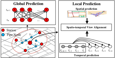
where Sl↪m is the geographical similarity between task (node) l and task (node) m, and measures the spatial autocorrelation between task l and m. Intuitively, if Sl↪m is large, the graph Laplacian regularizer term will force wl to be as similar as wm. Thus, this graph Laplacian penalty automatically encodes Toblers first law of geography [Tobler, 1970]. In implementation, we can pre-compute Sl↪m through the structure of pipe network. In particular, the pipe network can be seen as a weighted graph, where the weight for a pipe p is computed from its diameter p▷d, length p▷len and age p▷age by p▷d p▷len ⇤ p▷age. Given two stations Pl and Pm, as there are multiple different paths between Pl and Pm, their geographical similarity Sl↪m is computed by the sum of top-k shortest paths between them. λ↪ γ↪ ✓ are regularization parameters. The `2↪1-norm of a matrix W is defined as kWk2↪1 = PDi=1 qPMj=1 W 2 ij . In particular, `2↪1-norm applies an `2norm to each row of W and these `2-norms are combined through an `1-norm. As we assume that only a small set of features are predictive for a prediction task, the `2↪1-norm encourages all tasks to select a common set of features and thereby plays the role of group feature selection [Yuan and Lin, 2006]. Figure 3 illustrates the main idea of our approach.
5.3 Optimization
The optimization of Eqn.(3) is convex with respect to W. First, we can rewrite the graph Laplacian term in Eqn.(3) as
where D is a diagonal matrix with Dl↪l = Pm Sl↪m, S is the similarity matrix, and L = D - S is known as the Laplacian matrix. We define
The optimization in Eqn.(3) can be rewritten as minWh(W) + g(W), where h(W) is smooth and g(W) is non-smooth. We can thus use the Fast Iterative ShrinkageThresholding Algorithm (FISTA) [Beck and Teboulle, 2009] or Accelerated Gradient Descent [Nesterov, 2013] to solve it.
6 Experiments
6.1 Experimental Settings
Datasets
We evaluate our method with six datasets collected from August 2011 to August 2014 in Shenzhen City, China:
- ÷ Water quality data: We collected water quality data every five minutes from 15 water quality sites in Shenzhen City. It comprises Residual Chlorine (RC), turbidity and pH. In the experiment, we only use RC as the index for water quality.
- ÷ Hydraulic data: Hydraulic data consists of flow and pressure, which are collected every five minutes from 13 flow sites and 14 pressure sites, respectively.
- ÷ Road networks data: Each road segment is associated with two terminal points and some properties, such as level, capacity and speed limit.
- ÷ Pipe attributes data: It describes the pipe attributes in water distribution system, and the attributes of a pipe consist of diameter, length, age, material, etc.
- ÷ Meteorology data: Meteorological data consists of weather, temperature, humidity, barometer pressure, wind strength, which is collected every hour.
- ÷ POIs: There are 185,841 POIs of 20 categories. Each POI has a name, category, address and geo-coordinates.
Ground Truth and Metrics
We can predict the water quality of a site from its historical data, and the ground truth is obtained from its later readings. In particular, we evaluate the predictive performance with respect to its readings in next 1, 2, 3, 4 hours, and the performance is evaluated in terms of their root-mean-square-error (RMSE): RMSE = q 1N PMl=1 (yl - ˆyl)2 .
6.2 LearningModel Comparison
To validate our stMTMV model, we compared it with the following six baselines:
- ÷ RC Decay Model (Classical): Residual Chlorine (RC) decay model is a classical model in environmental science to model and predict chlorine residual in water supply systems [Monteiro et al., 2014; Rossman and Boulos, 1996]. This model describes both bulk and wall chlorine consumption via first order decay kinetics dC dt = -kC, where k is the first order chlorine decay constant that depends on the distribution systems.
- ÷ ARMA: Auto-Regression-Moving-Average (ARMA) is a well-known model for predicting time series data, which makes predictions solely based on historical data.
- ÷ LR: Linear Regression (LR) is applied for each node individually, which is a single-task learning method.
- ÷ LASSO: Lasso [Tibshirani, 1996] tries to minimize the objective function 12 PMl=1 kyl - Xlwlk22 + ↵kWk1 and encodes the sparsity over all weights in W. It keeps taskspecific features but ignores the task-sharing features.
- ÷ MRMTL: As a typical example of traditional multitask learning, Mean-Regularized Multi-Task Learning (MRMTL) [Evgeniou and Pontil, 2004] assumes all tasks are related and penalizes the deviation of each task from their mean by optimizing 12 PMl=1 kyl - Xlwlk22 + λ PMl=1 kwl - 1M PMm=1 wmk22 + ✓kWk2F .
- ÷ regMVMT: The regularizedmulti-viewmulti-task learning model (regMVMT) [Zhang and Huan, 2012] jointly regularizes view consistency and uniform task relatedness.
The experimental results are demonstrated in Table 1. From this table, we have the following observations: 1) The prediction accuracy of all models shows a decrease trend for the next four hours. This is consistent with the intuition that the distant future tends to be more difficult to forecast than the near future. 2) The last four multi-task learning methods outperform the first three single-task learning methods, which verifies that the tasks are not independent and capturing their relatedness can improve learning performance. Moreover, it is not unexpected that RC Decay Model achieves the worst performance since it may fail to capture the real dynamics of the RC in the system. 3) The accuracies of MRMTL are slightly lower than other multi-task learning methods. This may be caused by the inappropriate assumption of penalizing the deviation of each task from their mean, since these tasks tend to be spatially autocorrelated. 4) As compared to MTL, our model and regMVMT achieve higher performance due to the fact that stMTMV and regMVMT can incorporate heterogeneous information from spatial and temporal views, which may help to improve overall performance. 5) The stMTMV model shows superiority over regMVMT, which underscores the importance of incorporating structure of the water distribution system and this structure can further improve performance.
| Models | 1 hour | 2 hour | 3 hour | 4 hour |
|---|---|---|---|---|
| RC Decay Model | 3▷51e-1 | 3▷53e-1 | 3▷59e-1 | 3▷68e-1 |
| ARMA | 1▷86e-1 | 2▷18e-1 | 2▷46e-1 | 2▷78e-1 |
| LR | 1▷68e-1 | 1▷99e-1 | 2▷09e-1 | 2▷10e-1 |
| LASSO | 1▷23e-1 | 1▷42e-1 | 1▷52e-1 | 1▷56e-1 |
| MRMTL | 1▷32e-1 | 1▷48e-1 | 1▷56e-1 | 1▷58e-1 |
| regMVMT | 1▷06e-1 | 1▷15e-1 | 1▷18e-1 | 1▷19e-1 |
| stMTMV | 9.33e-2 | 9.66e-2 | 9.80e-2 | 9.90e-2 |
6.3 Evaluation onModel Components
To evaluate each component of the stMTMV model, we compared it with three different variants of stMTMV:
- ÷ stMTMV-us: In this variant, uniform spatial correlation is used to evaluate the importance of spatial correlation among tasks. We can derive it by setting S = I.
- ÷ stMTMV-ws: This is a derivation of stMTMV without group sparsity. We can derive it by setting ✓ = 0.
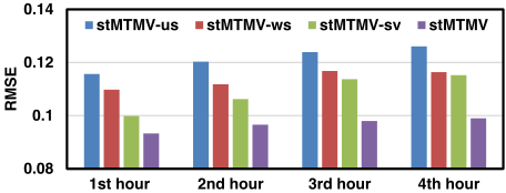
- ÷ stMTMV-sv: This derivation is to evaluate the importance of spatio-temporal view alignment. We can derive it by setting λ = 0.
The experimental results are demonstrated in Figure 4. From this figure, it can be seen that stMTMV-us achieves the worst performance, which demonstrates the effectiveness of graph Laplacian component in the stMTMV model.
This further verifies that the tasks are mutually correlated and the spatial autocorrelation plays an important role in the coprediction tasks. Moreover, stMTMV-ws achieves the second worst performance, which justifies the importance of group sparsity in the stMTMV model. This also provides evidence for the assumption that only a small set of features are predictive for the water quality prediction tasks. Compared to stMTMV-ws and stMTMV-us, the effect of spatio-temporal view alignment tend to be weaker, and this is observed by the superior performance of stMTMV-sv over other two variants. However, stMTMV outperforms stMTMV-sv since spatiotemporal view alignment can combine heterogeneous spatiotemporal information and further boost performance.
6.4 Evaluation on Views
To demonstrate the descriptiveness of each view, we compared our stMTMV model over the following combinations.
- ÷ t-view: Only temporal view (t-view) is used.
- ÷ s-view: Only spatial-view (s-view) is used.
- ÷ st-view-na: Both spatio-temporal views are used, but there is no s-t view alignment within each station.
- ÷ st-view: Both spatio-temporal view are used and the s-t view alignment is employed for each station.
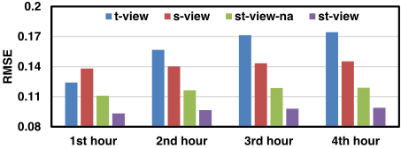
The results are presented in Figure 5. From this figure, we observe that: 1) the combinations of spatial and temporal views outperform each individual one. This observation reveals that the more views fed to our model, the better the performance will be. 2) the st-view outperforms st-viewna, which implies that aggregating information from spatial and temporal views can achieve better performance than concatenating them together. This also verifies that the heterogeneous information distributed across spatial and temporal views is usually complementary rather than conflicting, and appropriate aggregation of these can provide a better way to capture each station's characteristics comprehensively, and consequently boost the performance.
6.5 Water Quality Predictions
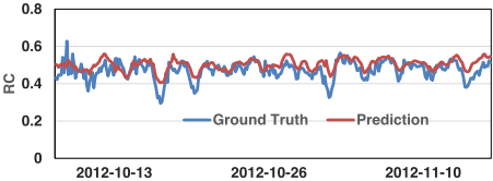
Figure 6 depicts the predictive results of our method over the next one hour against the ground truth in Shenzhen from October 2012 to November 2012. In general, our model is very accurate in tracing the ground truth curves (including sudden changes) of the water quality in Shenzhen City, which demonstrates the effectiveness of our approach.
6.6 Computational Complexity Analysis
In this section, we discuss the computational complexity for solving the stMTMV model. For the optimization of W, the complexity for each iteration in the FISTA algorithm is O((D + M)DM). Moreover, the FISTA algorithm converges within O(1◁✏2 ) iterations, and the total time cost of FISTA for solving stMTMV is O( (D+M)DM ✏2 ), where ✏ is the desired accuracy. Thus, the stMTMV model can be solved efficiently. Since the per-iteration complexity of FISTA for solving stMTMV is independent of N, which shows that our model can potentially scale to large-scale urban data.
7 RelatedWork
7.1 Classical Model-based Approaches
It is worth mentioning that several research efforts have been dedicated to model-based approaches for urban water quality prediction [Rossman et al., 1994; Monteiro et al., 2014; Rossman and Boulos, 1996]. The main idea behind this kind of approaches is to utilize the first-order or higher-order kinetics to model the chlorine decay along the water distribution system. However, the mechanisms of the chlorine decay is quite complicated, which comprise of reactions with bulk fluid, pipe and natural evaporation. Hence, the accurate mathematical modelling of chlorine decay along the water supply system is a tough problem that has not been fully solved [Castro and Neves, 2003]. Moreover, the developed decay model requires extensive human labors to perform model calibration with pipe networks, and it depends heavily on the pipe internal surface materials, temperatures, network structure, which makes it difficult to extend to other cities' water distribution systems. Compared to model-based approaches, datadriven based approaches demonstrate their advantages in both flexible and extendibility in many other ubiquitous applications [Zheng et al., 2014; Zheng, 2015; Liu et al., 2015; 2016a; Zheng et al., 2015b], such as urban air quality forecast [Zheng et al., 2015a], destination prediction [Xue et al., 2013; Zheng, 2015], and traffic prediction [Wang et al., 2014]. However, to the best of our knowledge, the literature on urban water quality prediction from the data-driven perspective is relatively sparse.
7.2 Multi-taskMulti-view Learning
Multi-task learning is a learning paradigm that jointly learns multiple related tasks and has demonstrated its advantages in many urban applications, such as transportation and event forecasting [Zhao et al., 2015; Zheng et al., 2014; Zhou et al., 2011]. In particular, it is more effective in handling those with insufficient training samples [Evgeniou and Pontil, 2004; Liu et al., 2015; 2016b; Zhou et al., 2011]. However, most of the existing approaches only explore the task relatedness, but ignore the consistency information among different views within a task. Multi-view learning has been proposed to leverage the information from diverse domains or from various feature extractors, and combining the heterogeneous properties from different views can better characterize objects and achieve promising performance [Zhang et al., 2013; Liu et al., 2016b; Zheng, 2015; Zheng et al., 2015b]. Nevertheless, existing multi-view learning approaches discard the label information from other related tasks, which usually leads to suboptimal performance. Thus, multi-view multi-task learning is proposed to explore both task relatedness and view relatedness simultaneously within a learning framework [Zhang and Huan, 2012; Liu et al., 2016b; He and Lawrence, 2011]. For example, He et al. [2011] proposed a graph-based iterative framework (GraM 2 ) for multi-view multi-task learning and obtained impressive results in text categorization applications. However, as far as we know, the literature on spatio-temporal based multi-task multi-view learning is relatively sparse. To the best of our knowledge, our approach is the first work on spatio-temporal based multi-task multi-view learning, which can incorporate spatio-temporal heterogeneities via a multi-task multi-view learning framework and is able to applied to other spatiotemporal based applications.
8 Conclusion and FutureWork
This paper presents a novel spatio-temporal multi-view multitask learning framework to forecast the water quality of a station by fusing multiple sources of urban data. It consists of two alignments. The first alignment is spaiotemporal view alignment. It works toward local information aggregation for each station. The second one is global prediction alignment, which incorporates the spatial correlations among stations and performs co-prediction over all stations using these correlations. Extensive experiments on real-world data show significant gains of these two alignments and their overall performance as compared to state-of-the-arts methods. The code has been released at: http://research.microsoft.com/apps/pubs/?id=264770.
In future, we will extend our model to learn the source confidence adaptively. Moreover, we will explore the problem of water quality inference through a limited number of monitor stations in the urban water distribution systems.
Acknowledgments
This work was supported by the China National Basic Research Program (973 Program, No. 2015CB352400), NSFC under grant U1401258, NSCF under grant No. 61572488. This research was also supported in part by grants R-252000-473-133 and R-252-000-473-750 from the National University of Singapore. We also thank Yipeng Wu for sourcing the data in this study.
@inproceedings{ijcai2016p366,
  title     = {Urban Water Quality Prediction Based on Multi-Task Multi-View Learning},
  author    = {Liu, Ye and Zheng, Yu and Liang, Yuxuan and Liu, Shuming and Rosenblum, David S.},
  booktitle = {Proceedings of the Twenty-Fifth International Joint Conference on
               Artificial Intelligence, {IJCAI-16}},
  publisher = {AAAI Press / International Joint Conferences on Artificial Intelligence},
  editor    = {Subbarao Kambhampati},
  pages     = {2576--2580},
  year      = {2016},
  month     = {7},
  url       = {https://ijcai.org/proceedings/2016/366},
}
TY - CPAPER TI - Urban Water Quality Prediction Based on Multi-Task Multi-View Learning AU - Liu, Ye AU - Zheng, Yu AU - Liang, Yuxuan AU - Liu, Shuming AU - Rosenblum, David S. T2 - Proceedings of the Twenty-Fifth International Joint Conference on Artificial Intelligence, IJCAI-16 PB - AAAI Press / International Joint Conferences on Artificial Intelligence PY - 2016 SP - 2576 EP - 2580 UR - https://ijcai.org/proceedings/2016/366 ER -Copied
Machine-readable versions of this paper, for tools and AI agents:





