Multi-View Embedding Learning for Incompletely Labeled Data

1 Introduction

Nowadays we are inundated with abundant data such as images, videos, documents, web pages, etc. The main characteristics of these datasets are as follows. i) High-dimension multi-view: For the low-level feature, the feature vector is high-dimensional and often includes multiple kinds of features, i.e., these features are in different spaces and thus heterogeneous; ii)Multi-concept incomplete-label: For the highlevel feature, one datum might be associated with more than one semantic concept simultaneously, and semantic richness requires multiple labels to sufficiently describe the datum; however, it is difficult to label the data without missing any concept, and generally the label information of each sample is incomplete. There is semantic gap between the input multi-view feature spaces (low-level) and the semantic concept space (high-level); and it is of significance to learn the bridge between the above spaces.

In real-world applications, there are many datasets with multiple views, that is, one datum point may be represented in several different feature spaces. For example, web images can be described by heterogenous features such as color descriptors, texture descriptors, shape descriptors, and the surrounding texts. Another example is the web categorization task where the web can be described by either the words occurring in web pages or the hyperlinks between web pages [Zhou and Burges, 2007]. We should consider learning from data with multiple views to effectively use multiple representations simultaneously, and such learning issue is usually called multiview learning. One approach to multi-view learning is cotraining [Kumar and Daume, 2011] where multiple learning algorithms are trained for each view and the relationship between a pair of points should be consistent across different views. [Zhou et al., 2007] takes advantage of the correlation between the views using CCA(Canonical Correlation Analysis) [Hotelling, 1936] and performs semi-supervised learning with only one labeled training sample. In [Zhou and Burges, 2007; Fu et al., 2011], multi-view spectral clustering is performed by generalizing Normalized Cut from the single view to the multi-view case, but they ignore the feature correlations between views. Other multi-view learning algorithms are included in [Harel and Mannor, 2011; Quadrianto and Lampert, 2011; Bronstein et al., 2010; Kumar and Udupa, 2011; Kumar et al., 2011; Dhillon et al., 2011a]. However, these methods do not take into account the correlation between concepts which will affect the performance in the multi-label setting.

Multi-label learning deals with the data associated with more than one concepts simultaneously and is often applied to image/video annotation, text categorization, web page classification, and so on. Multi-label learning has received many attentions in the field of machine learning recently, such as TagProp [Guillaumin et al., 2009], MBRM [Feng et al., 2004], ML-GRF [Zha et al., 2009], AFSVM [Chen et al., 2010], RankSVM [Elisseeff and Weston, 2002], RML [Petterson and Caetano, 2010] and references therein. In multi-label classification, the correlations between labels can be captured to improve the performance of classifiers. For example, the concepts camel and desert often co-occur in the same image, while panda and desert may seldom co-occur. Among various studies on multi-label learning, it is still unclear how to learn from multi-view data and how to capture inter-label correlations for embedding learning at the same time. In [Sun et al., 2011], some extensions of CCA(Canonical Correlation Analysis) are proposed for multi-view multi-label learning. One assumption in many multi-label learning algorithms is that for each training sample, all of its associated labels are provided completely, which may not hold in real applications however. In practice, it is hard to get all the proper labels, and usually the label information of samples is incomplete. For example, given one image containing the concepts bird, sky, cloud and tree, one may only label the image with bird and sky while missing cloud and tree. In this case, only an incomplete label set is available, and therefore, for some label which has not been assigned to the sample, the conclusion can not be drawn that this label is not proper for the sample. The existing methods on incompletely labeled data include [Lee and Liu, 2003; Sun et al., 2010; Lu et al., 2012; Liu et al., 2010a; Chen et al., 2010; Wang et al., 2007]; above methods only allows for inter-label correlations but not for inter-feature correlations because they are not developed for multi-view data.

Embedding learning is a popular approach to deal with high-dimensional data, which assumes that all data points reside on an intrinsic manifold and find its embedding in a low-dimensional space. In the past years many algorithms on embedding learning have been proposed [Roweis and Saul, 2000; Belkin and Niyogi, 2001; He et al., 2005; Chen et al., 2005], but they are not designed for multi-view multi-label learning. In [Dhillon et al., 2011b], a learning method is presented to estimate low dimensional contextspecific word representations from unlabeled data using a spectral method; [Zhang and Zhou, 2010] performs multilabel dimensionality reduction by maximizing the dependence between the original feature description and the associated class labels; however, it is not clear how to exploit the weak supervised information in the incomplete label problem.

In this paper we propose a novel method to learn compact embedding that captures inter-feature correlations, interlabel correlations, and feature-label associations simultaneously from multi-view incompletely-labeled data. Each datapoint is represented by heterogeneous features in different spaces, so multi-view learning is performed to obtain the optimal combined features which exploit the feature correlations across different views. We assume that data are in three kinds of spaces: i) multiple input feature spaces, ii) compact embedding space, and iii) a semantic concept space. By mapping data frommultiple input feature spaces to the embedding space and to the concept space, we seek the embedding which preserves the neighborhood context in the original spaces, and complete the labels at the same time. There is semantic gap between the input multi-view feature space and the semantic concept space; and the compact embedding space can be looked on as the bridge between the above spaces. Each data-point is associated with more than one semantic concepts, so inter-label relations are exploited for embedding learning. The proposed method is weakly supervised because the label information available is incomplete.

The rest of this paper is organized as follows: In Section 2 we formulate the proposed model for embedding learning from multi-view incompletely-labeled data. Our experimental results on real datasets are given in Section 3. Finally, we conclude this paper in Section 4.

2 The ProposedMethod

Suppose that there are n incompletely labeled samples: X = [x1, x2, ..., xn], among which each is represented by multiple heterogeneous features; Y = [y1, ..., yn] ∈ {0, 1}c×n , where yu ∈ {0, 1}c is the label vector of the incompletely labeled sample xu, (u = 1, ..., n) and c is the number of labels considered. ylu = 1(l = 1, . . . , c) indicates that the l-th label is a proper label for xu, while ylu = 0 tells us nothing (i.e., the absence of a label does not mean that it is not appropriate for the sample). In the multi-label scenario, one datum may be associated with multiple concepts simultaneously, thus there may be more than one positive elements in the c-dimensional binary vector yu. Let H = [h1, ..., hn] ∈ Rr×n denote the embedding for all n samples in the r-dimensional space, and the u-th column hu corresponds to the embedding code for the sample xu. We try to seek the compact embedding and to complete the labels of all data-points represented by heterogeneous features in a unified framework. Intuitively, assume that data points lie on a r-dimensional manifold embedded in multiple input feature spaces, our goal is to find the maps from multiple input spaces to the compact embedding space and to the semantic concept space at the same time. It is worthy to note that the multiple input feature spaces are heterogeneous; there is semantic gap between the input multi-view feature space and the semantic concept space; and the compact embedding space can be looked on as the bridge between the above spaces.

2.1 Multi-View Learning with Heterogeneous Features

For multi-view data , it is of significance how to identify the similarity between samples represented by multiple features. Suppose that each datum is represented by J heterogeneous features, and we define J 2 directed graphs Gij = (V,Wij), i, j = 1, ..., J over the dataset, where V is the set of nodes and each node represents one sample; Wij = [wij(u, v)]n×n is the weight matrix and wij (u, v) measures the similarity between samples xu and xv from the i-th and the j-th views, respectively. It should be pointed out that these graphs share the same set of nodes while having different similarity matrices for different pair of views. With respect to the view pair (i, j), the volume of graph Gij is volijV = ∑u∈V,v∈V wij(u, v). The natural random walk on Gij can be defined as follows. That is, given a node u, we try to walk from u to v, and the transition probability on Gij is p(u → v|Gij, u) = wij(u, v)/∑v∈V wij(u, v) and the probability of u on Gij is p(u|Gij) = ∑v∈V wij(u, v)/volijV . Let p(Gij) denote the prior probabilities of the random walker choosing the graph Gij(1 ≤ i, j ≤ J), and we have p(Gij) ≥ 0 and ∑ij p(Gij) = 1. Then the probability of node u on multiple graphs is computed as p(u) = ∑ij p(u|Gij)p(Gij).

According to Bayes' theorem, the posterior probability to choose the graph Gij at node u is p(Gij|u) = p(u|Gij )p(Gij ) ∑ij p(u|Gij)p(Gij) . Thus, for any node u, the transition probability of u → v on multiple graphs can be computed as p(u → v|u) = ∑ij p(u → v|Gij , u)p(Gij |u). Observe that

where wii(u, v) = exp{-γ‖x(i) u -x(i) v ‖2}measures the similarity between samples represented by the features in the same view, and wij(u, v)(i ̸= j) measures the similarity between samples across different views. We use CCA technique to define wij (u, v)(i ̸= j) which captures the correlations between heterogeneous feature spaces.

Let X(i) = [x(i) 1 , ..., x(i) n ] and X(j) = [x(i) 1 , ..., x(j) n ] denote the dataset from the i-th and the j-th views, respectively. Assume that they are firstly centered such that ∑nv=1 x(i) u = 0 and ∑nv=1 x(j) u = 0. The covariance matrices are denoted as follows: Cii = X(i)X(i)⊤, Cjj = X(j)X(j)⊤, Cij = X(i)X(j)⊤, and Cji = X(j)X(i)⊤. Canonical Correlation Analysis (CCA) is employed to learn the common space to compute the similarity between samples from multi-view spaces. More specifically, the projection directions where samples are most correlated are firstly learned by max{φi ,φj } φi⊤Cijφj √φi⊤Ciiφi φj⊤Cjjφj , which is equivalent to seeking the eigenvectors w.r.t. largest eigenvalues of Cii-1CijCjj -1Cji and Cjj -1CjiCii-1Cij, respectively.

Denote T = Cii- 12 CijCjj - 12 . TT ⊤ and T ⊤T are both symmetric positive semi-definite and share ˜ r positive eigenvalues λ1, ..., λ˜ r, herein ˜ r = rank(TT ⊤) = rank(T ⊤T). Since Cii-1CijCjj -1Cji = Cii- 12 TT ⊤Cii 1 2 and Cjj -1CjiCii-1Cij = Cjj - 1 2 T ⊤T Cjj 12 , Cii-1CijCjj -1Cji and Cjj -1CjiCii-1Cij are similar to TT ⊤ and T ⊤T respectively. Thus, Cii-1CijCjj -1Cji and Cjj -1CjiCii-1Cij also share the above r positive eigenvalues λ1, ..., λ˜ r. Denote Λ = diag(λ1, ..., λ˜ r ), Φi = [φi1 , ..., φi˜ r ], and Φj = [φj1 , ..., φj˜ r ]. Because Cii-1CijCjj -1CjiΦi = ΦiΛ and Cjj -1CjiCii-1CijΦj = Φj Λ, so TT ⊤Cii 1 2 Φi = Cii 12 ΦiΛ and T ⊤TCjj 12 Φj = Cjj 1 2 Φj Λ. Suppose that Ψ and ˜Ψ are the sets of orthonormal eigenvectors with respect to r positive eigenvalues for TT ⊤ and T ⊤T respectively. Then we can easily calculate the transformation matrix Φi = Cii- 12 Ψ and Φj = Cjj - 1 2 ˜Ψ. The transformed data Φi⊤X(i) and Φj⊤X(j) are in a common ˜ r-dim feature space, where the correlation matrix is Λ 12 . Thus the similarity between samples across different views wij(u, v)(i ̸= j) in Eq. (1) can be defined as wij(u, v) = exp{-σ‖Φi⊤x(i) u - Φj⊤x(j) v ‖2 }. Note that wii(u, v) = wii(v, u), while wij(u, v) ̸= wij(v, u), (i ̸= j). However, ∑i̸=j wij (u,v) volijV p(Gij) = ∑j̸=i wji(u,v) voljiV p(Gji) , thus we have p(u)p(u → v|u) = p(v)p(v → u|v) =: w(u, v), which can be defined as the similarity measurement for the data points in multiple views.

2.2 Embedding Learning for Incompletely Labeled Data

Based on the above random walk process among multiple graphs, we can seek the compact embedding of multi-view data and predict the labels in a unified framework. Let ˆY = [ˆy1, ..., ˆyn] ∈ {-1, 1}c×n denote the label prediction matrix for all the samples where ˆylu = -1 means that the lth label is not a correct label for xu. ˆY can be investigated from different perspectives: i)column view: Each column of ˆY corresponds to the estimated label vector for one data, and can be viewed as the high-level feature vector of the u-th sample in the semantic label space, which differs from the lowlevel feature vectors in the visual feature spaces; ii)row view: Each row of ˆY can be viewed as the voting scores from all the samples for each concept, and can also be viewed as the feature vector of the concept. By leveraging the information from above two perspectives, we can sufficiently capture the semantic context, and the neighborhood consistency between input spaces and embedding space in the proposed framework formulated as follows:

where col( ˆY, u) denotes the u-th column of the matrix ˆY, which is the estimated multi-label vector for the sample xu; row( ˆY, s) denotes the s-th row of the matrix ˆY, which indicates for the s-th concept which samples are positive while the others are negative. Solving Eq. (2) is difficult and we can relax the domain of ˆY from {-1, 1}c×n to [-1, 1]c×n . ρ(s, t) is defined to capture the correlations between concepts s and t. θ1 and θ2 are the tradeoff parameters.

Intuitively, the first term in the objective function Eq. (2) forces the label prediction to fit the given labels as much as possible. Since yu ∈ {0, 1}c , the penalty occurs only when ylu = 1, and y⊤ u (yu - col( ˆY, u)) = ∑cl=1 ylu (1 - ˆylu ) ≥ 0.

The second term constrains that the difference of embedding codes between samples should be as small as possible when they are strongly connected(i.e., with high transition probability). It is reasonable to preserve the neighborhood contexts when mapping from the input feature spaces to the embedding space. The third term achieves that strongly correlated concepts should have similar voting scores from all the samples. The correlation between concepts ρ(s, t) can be initialized as the harmonic mean of the empirical conditional probabilities:ρ(s, t) = 2p(t|s)p(s|t) p(t|s)+p(s|t) , where the empirical conditional probability p(t|s) = ∑lu=1 (ysu )(ytu ) 2 ∑lu=1 (ysu ) is derived from the labeled samples and measure the co-occurrence of concept pair on the given data. ( ysu = 1(s = 1, . . . , c) means that the s-th concept is associated with the u-th sample, while ysu = 0 tells nothing.)

Suppose that each datum xu represented by multiple features is firstly nonlinearly mapped to the r-dimensional embedding space hu = φ(xu), and then the label vector can be estimated by mapping hu to the c-dimensional semantic concept space using the discriminant function ˆyu = Qhu, where Q ∈ Rc×r is the linear transformation matrix. Denote ˆY = QH = Q[h1, ..., hn], which is the label prediction matrix for all the samples. Above maps from heterogeneous feature spaces to embedding space and to concept space over multiple graphs can be learned in Eq. (2) as

where row(Q, s) denotes the s-th row of the matrix Q. By introducing the Laplacian matrices we can rewrite Eq. (3) as

where the matrices Lρ and Lw are two different graph Laplacians. More specifically, Lρ = D - F, where F = [ρ(s, t)]c×c and D is a diagonal matrix with D(s, s) = ∑t ρ(s, t). Let G′ = ({s}cs=1 , F) denote the semantic context graph with the vertex set corresponding to the concepts {s}cs=1 and the weight matrix F measuring the correlations between concepts, thus Lρ is the graph Laplacians over G′ = ({s}cs=1 , F ) modeling the semantic context. Likewise, let ˜G = (V,W) denote the multi-graph with the edge weight matrix W = [w(u, v)]n×n derived by natural random walk over multiple graphs and let Λ be a diagonal matrix with Λ(u, u) = ∑v w(u, v), thus Lw = Λ-W is the multi-graph Laplacian modeling the consistency between neighborhoods in the embedding space and those in multi-view input feature space.

As pointed out before, ρ(s, t) can be initialized by the empirical conditional probabilities using the given labeled dataset, then Lρ is estimated initially as well. The correlations between concepts derived by the empirical conditional probabilities is simple and effective if the samples are completely labeled. For incompletely labeled dataset, the empirical conditional probabilities might not be estimated correctly, thus ρ(s, t) and Lρ are not expected to capture the semantic context relationship well. To address this problem, we can learn semantic context, embedding codes, and the label confidence vectors simultaneously by modifying the framework Eq. (4) as minQ,H,Lρ f, and we can obtain the solutions in an iterative way. We minimize the cost function Eq. (4) by updating H, Q, and Lρ alternatively. We derive the gradients of the above cost function with respect to H, Q, and Lρ, respectively:

Then the optimal H, Q, and Lρ can be iteratively learned in an alternating updating way as follows:

where α, β and γ (0 < α, β, γ < 1) are all the step sizes for gradient search. Based on the available incomplete label matrix Y = [y1, ..., yn] ∈ {0, 1}c×n , we employ the technique called Non-negative Matrix Factorization(NMF)[Lee and Seung, 1999] to initialize H and Q: Y = Q0H0 . Once the optimal H and Q are learned, the optimal label prediction matrix for all the samples is computed straightforward ˆY = QH, and we can predict the label vectors easily by choosing a threshold for each row of ˆY.

2.3 Discussion

It is worthy to note that the Laplacian matrix Lw in Eq. (4) is n × n, and the complexity of Eq. (4) is high over large dataset. For scalability, we can also learn an approximate matrix for the Laplacian Lw like[Liu et al., 2010b]. Specially, clustering is firstly performed on n data points to obtain m(m >> n) anchor points. The weight between the non-anchor point u and the neighboring anchor v is defined as Zuv = w(u,v) ∑j∈〈v〉 w(j,v) , where 〈v〉 denotes the indices of nearest anchors of point v. Zuv = 0 if u /∈ 〈v〉, so the weight matrix Z ∈ Rm×n is highly sparse. We only need to solve the embedding codes associated with anchors which are put in the matrix A ∈ Rr×m in which each column vector accounts for one anchor. Then the embedding for all data can be computed easily by H = AZ. Substitute H with H = AZ in Eq. (4), we can easily learn the optimal A in the iterative way as before. It should be pointed out that the second item in Eq. (4) becomes Tr(AZLwZ ⊤A⊤). Based on the random walks across data points and anchors, the approximation to the Laplacian matrix is derived as Lw = I - Z ⊤Λ-1Z, where Λ = diag(Z1) ∈ Rm×m. Thus, ZLwZ ⊤ = ZZ ⊤ - ZZ ⊤Λ-1ZZ ⊤ , which is both memory-wise and computationally tractable, and the second item in Eq. (4) becomes Tr(AZZ ⊤A⊤ - AZZ ⊤Λ-1ZZ ⊤A⊤). Furthermore, learning the embedding for anchors enables efficient out-of-sample extension. For any novel datum point, the embedding can be computed as φ(x) = Az(x) where z(x) is m-dim weigh vector whose u-th element is z(u, x) = w(u,x) ∑j∈〈x〉 w(j,x) .

3 Experiments

We experimentally evaluate the performance of the proposed method, denoted by ′ ours′ , and compare it with WELL [Sun et al., 2010] and PUWLR [Lee and Liu, 2003]. PUWLR [Lee and Liu, 2003] is a method learning with Positive and Unlabeled data using Weighted Logistic Regression; WELL (WEak Label Learning) [Sun et al., 2010] is the method designed for incompletely labeled dataset. Furthermore, we also evaluate the degenerated version of our method denoted by ′ ours-′ where the multiple heterogeneous features are simply concatenated into a high-dimensional vector without capturing inter-feature correlations. We conduct experimental evaluations on three image datasets: MSRC [Shotton et al., 2006], LabelMe [Russell et al., 2008] and NUS-WIDE [Chua et al., 2009].

3.1 Results onMSRC

MSRC image dataset [Shotton et al., 2006] is widely used in multi-label learning for performance evaluation. It contains 591 photographs with 23 concepts in total. We ignore the concepts horse and mountain since they have few instances. Thus there are totally 21 concepts in our experiments. About 80% images are associated with multiple labels. There are about 3 labels on average per image. Only one label per image is used for models training in the experiments such that MSRC can be employed as the incompletely labeled data. For each image, we extract five kinds of features: 12-dim CLD (Color Layout Descriptor), 64-dim SCD (Scalable Color Descriptor), 256-dim CSD (Color Structure Descriptor), 80-dim EHD (Edge Histogram Descriptor), and 1024-dim SIFT feature.

Fig. 1 shows the experimental results of our method in comparison with other related methods on MSRC image dataset. We use four criterions to evaluate the performance: Macro-F1, Micro-F1, Hamming Loss and Ave-AUROC (Average Area Under ROC). As for the criterions Macro-F1, Micro-F1, and Ave-AUROC, the larger the value is, the better the performance is; meanwhile, as for Hamming Loss, the smaller, the better. It can be seen that our method consistently performs better than other methods in terms of these criterions. Our method sufficiently leverages inter-feature correlation, inter-label correlation, and feature-label association at the same time, which inherits all merits of the stateof-the-art methods. Note that the degenerated version of our method ′ ours-′ still performs better than or comparable with others because ′ ours-′ effectively captures the inter-label correlation from the incompletely labeled data, even though ′ ours-′ simply concatenates into a high-dimensional vector like WELL and PU WLR.

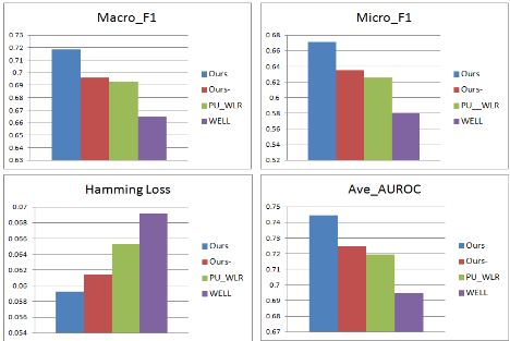
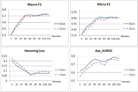
Fig. 2 illustrates the performance variations on different dimensions of the learned embedding space. As can be seen, the performance increases rapidly with the embedding dimensions are added at the first stage, and it tends to be stable afterward; it even turns to drop when longer codes are used. Thus the longest embedding code can not guarantee the best performance.

3.2 Results on LabelMe

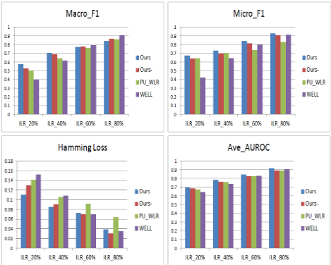
LabelMe image dataset [Russell et al., 2008] is dynamic, free to use, and open to public contribution. We choose a subset of the LabelMe dataset containing the top 33 object categories and totally 1,105 images. In this subset each image has more than 5 labels, and the average number of labels per image in this subset is 6.63. For the purpose of evaluation on incompletely labeled dataset, we present the ground truth of the labels for images in a full label matrix ˙Y = [ ˙y1, ..., ˙yn] ∈ {-1,+1}c×n where ˙ylu = +1 indicates the l-th label is a correct label while ˙ylu = -1 indicates the l-th label is not a proper label for the u-th image. We vary the Incomplete Label Ratio ( ILR, defined as the ratio of the available label number to the ground-truth ∑l 1{ylu = 1}/ ∑l 1{ ˙ylu = 1}) of each image from 20% to 80% with 20% as interval to study the performance of our method over various incompletely labeled data. For each image, we also extract five kinds of features: CLD, SCD, CSD, EHD, and SIFT. Fig. 3 shows the experimental results of our method in comparison with other related methods on LabelMe image dataset. Our method outperforms the state-ofthe-art methods in most cases.

3.3 Results on NUS-WIDE

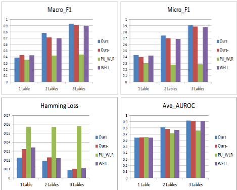
NUS-WIDE dataset [Chua et al., 2009] is a challenging collection of 269,648 images and the associated tags from Flickr, with a total number of 5,018 unique tags. Like [Liu et al., 2010a], we select a subset of NUS-WIDE dataset, focusing on images containing at least 5 labels, containing 19,277 images with 81 labels in total. In the experiments, only k (k=1,2,3) label per image are used for models training such that this dataset can be employed as the incompletely labeled data for evaluation. For each image, five types of low-level features are extracted: 144-Dim color correlogram, 73-Dim edge direction histogram, 128-Dim wavelet texture, 225-Dim block-wise color moments, and 500-Dim bag of words based on SIFT descriptions. All these features of NUS-WIDE images are available on web 1 and can be downloaded freely.

Fig. 4 gives the experimental results of our method in comparison with other methods on NUS-WIDE images. In the case that only one label per image is available, the performance of our method is comparable to that of the others on Macro-F1 and Ave-AUROC, and is better on Hamming Loss and Micro-F1. In the case that two or three labels per image are available, the proposed method outperforms the others consistently on these four criterions.

1 http://lms.comp.nus.edu.sg/research/NUS-WIDE.htm

4 Conclusions

In this paper we propose a novel method to learn compact embedding that captures inter-feature correlations, interlabel correlations, and feature-label associations simultaneously from multi-view incompletely-labeled data. Multiple directed graphs are constructed over the dataset to model different similarity matrices across views. We use CCA technique to capture the correlations between heterogeneous feature spaces. By mapping data from multiple feature spaces to the embedding space and further to the concept space, we learn the embedding which preserves the neighborhood context in the original spaces, and complete the labels at the same time. There exists semantic gap between the input multi-view feature spaces and the semantic concept space; and the compact embedding space can be looked on as the bridge over the gap between the above spaces.

Acknowledgments

We would like to thank the anonymous reviewers for their helpful comments. This work was supported in part by the Shanghai Leading Academic Discipline Project (No.B114), the STCSM's Programs (No. 12XD1400900), the NSF of China (No.60903077), and the 973 Program (No.2010CB327906).