
Connecting Qualitative Spatial and Temporal Representations by Propositional Closure
Proceedings of the Twenty-Fifth International Joint Conference on Artificial Intelligence. Pages 1308-1313.
© 2016 International Joint Conferences on Artificial Intelligence
Abstract
This paper establishes new relationships between existing qualitative spatial and temporal representations. Qualitative spatial and temporal representation (QSTR) is concerned with abstractions of infinite spatial and temporal domains, which represent configurations of objects using a finite vocabulary of relations, also called a qualitative calculus. Classically, reasoning in QSTR is based on constraints. An important task is to identify decision procedures that are able to handle constraints from a single calculus or from several calculi. In particular the latter aspect is a longstanding challenge due to the multitude of calculi proposed. In this paper we consider propositional closures of qualitative constraints which enable progress with respect to the longstanding challenge. Propositional closure allows one to establish several translations between distinct calculi. This enables joint reasoning and provides new insights into computational complexity of individual calculi. We conclude that the study of propositional languages instead of previously considered purely relational languages is a viable research direction for QSTR leading to expressive formalisms and practical algorithms.
- [Aiello et al., 2007] Marco Aiello, Ian E. Pratt-Hartmann, and Jo- han F.A.K. van Benthem, editors. Handbook of Spatial Logics. Springer, 2007.
- [Allen, 1983] James F. Allen. Maintaining knowledge about tem- poral intervals. Commun. ACM, 26(11):832-843, 1983.
- [Balbiani et al., 1998] Philippe Balbiani, Jean-Franc ¸ois Condotta, and Luis Fariñas del Cerro. A model for reasoning about bidi- mensional temporal relations. In Proc. of KR-98, pages 124-130.
- Morgan Kaufmann, 1998.
- [Barrett et al., 2008] Clark Barrett, Roberto Sebastiani, Sanjit A. Seshia, and Cesare Tinelli. Satisfiability modulo theories. In Armin Biere, Marijn Heule, Hans van Maaren, and Toby Walsh, editors, Handbook of Satisfiability. IOS Press, 2008.
- [Bodirsky and Kára, 2010] Manuel Bodirsky and Jan Kára. The complexity of temporal constraint satisfaction problems. Jour- nal of the ACM, 57(2), 2010.
- [Collins, 1974] George Collins. Quantifier elimination for real closed fields by cylindrical algebraic decompostion. ACM SIGSAM Bulletin, 8(3):80-90, 1974.
- [Condotta, 2000] Jean-Franc ¸ois Condotta. Tractable sets of the generalized interval algebra. In Proc. of ECAI 2000, pages 78- 82. IOS Press, 2000.
- [Fargier et al., 2013] Hélène Fargier, Pierre Marquis, and Alexan- dre Niveau. Towards a knowledge compilation map for heteroge- neous representation language. In Proceedings of the 23rd Inter- national Joint Conference on Artificial Intelligence (IJCAI 2013), 2013.
- [Fenelon et al., 2012] Valquiria Fenelon, Paulo E. Santos, Han- nah M. Dee, and Fabio G. Cozman. Reasoning about shadows in a mobile robot environment. Appl. Intell., 22(2), 2012.
- [Freksa, 1992a] Christian Freksa. Temporal reasoning based on semi-intervals. Artif. Intell., 54(1):199-227, 1992.
- [Freksa, 1992b] Christian Freksa. Using orientation information for qualitative spatial reasoning. In Spatio-Temporal Reasoning, vol- ume 639 of LNCS, pages 162-178. Springer, 1992.
- [Galton, 1994] Antony P. Galton. Lines of sight. In Proc. of AI and Cognitive Science '94, pages 103-113, 1994.
- [Jonsson and Bäckström, 1998] Peter Jonsson and Christer Bäckström. A unifying approach to temporal constraint reasoning. Artificial Intelligence, 102(1):143-155, 1998.
- [Koubarakis, 2001] Manolis Koubarakis. Tractable disjunctions of linear constraints: basic results and applications to temporal rea- soning. Theoretical Computer Science, 266:311-339, 2001.
- [Kreutzmann and Wolter, 2014] Arne Kreutzmann and Diedrich Wolter. Qualitative spatial and temporal reasoning with AND/OR linear programming. In Proc. of ECAI 2014, volume 263 of FAIA, pages 495-500. IOS Press, 2014.
- [Lee et al., 2013] Jae Hee Lee, Jochen Renz, and Diedrich Wolter. StarVars-effective reasoning about relative directions. In Proc. of IJCAI 2013, pages 976-982. AAAI Press, 2013. IJCAI
- [Lifschitz, 2008] Vladimir Lifschitz. What is answer set program- ming? In Dieter Fox and Carla P. Gomes, editors, Proceed- ings of the Twenty-Third AAAI Conference on Artificial Intel- ligence, AAAI 2008, Chicago, Illinois, USA, July 13-17, 2008, pages 1594-1597. AAAI Press, 2008.
- [Ligozat and Renz, 2004] Gérard Ligozat and Jochen Renz. What is a qualitative calculus? A general framework. In Proc. of PRI- CAI 2004, pages 53-64, 2004.
- [Ligozat, 1998] Gérard Ligozat. Reasoning about cardinal direc- tions. J. Vis. Lang. Comput., 9(1):23-44, 1998.
- [Liu et al., 2010] Weiming Liu, Xiaotong Zhang, Sanjiang Li, and Mingsheng Ying. Reasoning about cardinal directions between extended objects. Artif. Intell., 174(12-13):951-983, 2010.
- [Moratz and Ragni, 2008] Reinhard Moratz and Marco Ragni. Qualitative spatial reasoning about relative point position. J. Vis. Lang. Comput., 19(1):75-98, 2008.
- [Moratz and Wallgrün, 2012] Reinhard Moratz and Jan Oliver Wallgrün. Spatial reasoning with augmented points: Extending cardinal directions with local distances. J. Spatial Information Science, 5(1):1-30, 2012.
- [Mossakowski and Moratz, 2012] Till Mossakowski and Reinhard Moratz. Qualitative reasoning about relative direction of oriented points. Artif. Intell., 180-181:34-45, 2012.
- [Navarrete et al., 2013] Isabel Navarrete, Antonio Morales, Guido Sciavicco, and M. Antonia Cárdenas Viedma. Spatial reasoning with rectangular cardinal relations -the convex tractable subal- gebra. Ann. Math. Artif. Intell., 67(1):31-70, 2013.
- [Pujari et al., 1999] Arun K. Pujari, G. Vijaya Kumari, and Abdul Sattar. INDU: An interval and duration network. In Proc. of AI 1999, volume 1747 of LNCS, pages 291-303. Springer, 1999.
- [Ragni and Scivos, 2005] Marco Ragni and Alexander Scivos. De- pendency calculus: Reasoning in a general point relation alge- bra. In Proc. of KI 2005, volume 3698 of LNCS, pages 49-63. Springer, 2005. IJCAI
- [Randell et al., 1992] David A. Randell, Zhan Cui, and Anthony G. Cohn. A spatial logic based on regions and "Connection". In Proc. of KR 1992, pages 165-176.
- Morgan Kaufmann, 1992.
- [Renz and Mitra, 2004] Jochen Renz and Debasis Mitra. Qualita- tive direction calculi with arbitrary granularity. In Proc. of PRI- CAI 2004, pages 65-74, 2004.
- [Renz, 2001] Jochen Renz. A spatial odyssey of the interval alge- bra: 1. directed intervals. In Proc. of IJCAI 2001, pages 51-56. IJCAI
- Morgan Kaufmann, 2001.
- [Renz, 2002] Jochen Renz. Qualitative Spatial Reasoning with Topological Information, volume 2293 of LNCS. Springer, Berlin, 2002.
- [Scivos and Nebel, 2005] Alexander Scivos and Bernhard Nebel. The Finest of its Class: The Natural Point-Based Ternary Cal- culus LR for Qualitative Spatial Reasoning. In Spatial Cogni- tion IV. Reasoning, Action, Interaction, pages 283-303. Springer Berlin Heidelberg, January 2005.
- [Skiadopoulos and Koubarakis, 2005] Spiros Skiadopoulos and Manolis Koubarakis. On the consistency of cardinal direction constraints. Artif. Intell., 163(1):91-135, 2005.
- [Tarquini et al., 2007] Francesco Tarquini, Giorgio De Felice, Paolo Fogliaroni, and Eliseo Clementini. A qualitative model for visibility relations. In Proc. of KR 07, volume 4667 of LNCS, pages 510-513. Springer, 2007.
- [Vilain and Kautz, 1986] Marc B. Vilain and Henry A. Kautz. Con- straint propagation algorithms for temporal reasoning. In Proc. of AAAI 1986, pages 377-382.
- Morgan Kaufmann, 1986.
- [Westphal and Wölfl, 2009] Matthias Westphal and Stefan Wölfl. Qualitative CSP, finite CSP, and SAT: Comparing methods for qualitative constraint-based reasoning. In Proceedings of the 21th International Joint Conference on Artificial Intelligence (IJCAI 2009), 2009. IJCAI
- [Wölfl and Westphal, 2009] Stefan Wölfl and Matthias Westphal. On combinations of binary qualitative constraint calculi. In Pro- ceedings of the 21th International Joint Conference on Artificial Intelligence (IJCAI 2009), 2009. IJCAI
- [Wolter and Lee, 2010] Diedrich Wolter and Jae Hee Lee. Qualita- tive reasoning with directional relations. Artificial Intelligence, 174(18):1498-1507, 2010.
References were extracted automatically from the PDF and may contain errors.
Full text extracted automatically from the PDF; figures, tables and equations may differ. The PDF is the version of record.
1 Introduction
The field of qualitative spatial and temporal representation and reasoning (QSTR) draws its motivation from several application contexts. Qualitative representations employ a relational language to state relations between spatial or temporal entities, using a finite and often small vocabulary of concepts. Practitioners may design a qualitative representation to capture human-like concepts without being concerned about the computational effects of design decisions, while theoretical works aim to fathom the dependencies between domain representation and computational complexity of the resulting representation. Renz [2002] claimed that computational aspects in QSTR are under-explored and the claim may be regarded as valid up to today since not all representations proposed so far have been analyzed yet.
A more prevailing problem in QSTR stems from the contrast that a high specificity of a qualitative representation fos-
Jae Hee Lee
QCIS, FEIT University of Technology Sydney Australia
jaehee.lee@uts.edu.au
ters efficient reasoning algorithms, but applications often require considerations of several aspects at the same time, for example a robot reasoning about its relative orientation within its working environment as well as the arrangement of objects in the environment in terms of cardinal directions. To master this requirement, not only is a deep understanding of computational properties required, but we need to understand the interdependency of distinct formalisms.
In this paper we address the challenge from a point of view that is helpful for applications: we identify mappings between formalisms that allow statements in one formalism to be translated into another, retaining reference to the same domain objects. We particularly consider a class of mappings that rewrites relations from one formalism as Boolean combination of relations in the other formalism. This approach often does not affect the computational complexity class since most formalisms are at least NP-complete, but it allows expressive power to be increased and several translations to be established.
The approach taken in this paper is related to, but more general than the approaches of Kreutzmann and Wolter [2014] and Jonsson and B¨ackstr¨om [1998] that consider translations to disjunctions of linear inequalities and the approach by Westphal and W¨olfl [2009] that considers translations of qualitative constraint problems to SAT. In contrast to the previous works (i) we consider translations between any reasoning algorithm capable of handling a specific qualitative calculus and (ii) we are also involved with propositional closures, which are more expressive. We expect that studying the propositional closure of calculi is also valuable for research in spatial logics [Aiello et al., 2007], which take a broader perspective on logic formalisms in spatial and temporal reasoning. In this broader view, first-order definable relations are often studied and several full complexity classifications exist in many cases, most notably the case of temporal constraints definable in hQ↪ <i [Bodirsky and K´ara, 2010]. Thus, this paper focuses on an intermediate level between qualitative constraint calculi and first-order or algebraic constraint languages.
The remainder of this paper is organized as follows. Section 2 defines and introduces qualitative representations of space and time, their propositional closure, and introduces translations. Section 3 then establishes translations by giving proof sketches. Readers interested in the results may advance to Section 4 where we summarize the results of this paper, followed by a conclusion discussing the impact on future research in the field.
| Abbreviation, Name | Reference | Base entity | Aspect | Example statement | |
|---|---|---|---|---|---|
| Temporal | PC, Point Calculus DepCalc, Dependency Calculus IA, Allen's Interval Algebra INDU SIC GenInt, Generalized IA DIA, Directed Intervals Algebra | [Vilain and Kautz, 1986] [Ragni and Scivos, 2005] [Allen, 1983] [Pujari et al., 1999] [Freksa, 1992a] [Condotta, 2000] [Renz, 2001] | point in n-d point intervals in 1-d intervals in 1-d semi-intervals in 1-d tuples of intervals directed 1-d intervals | total order partial order total order order & duration total order total order order/orientation | x < y joint past of x and y x overlaps with y shorter x meets longer y x ends after y x before and after y x overlaps from behind= y |
| CDC, Cardinal Dir. Calc. BA, Block Algebra CDR, Cardinal Direction Rel's. RCD, Rectangle Cardinal Dir. STAR | [Ligozat, 1998] [Balbiani et al., 1998] [Skiadopoulos and Koubarakis, 2005] [Navarrete et al., 2013] [Renz and Mitra, 2004] | point in n-d n-d bounding box simple regions in 2-d simple regions in 2-d points in 2-d | total order total order direction direction direction | x below y x overlaps y at top x N and W of y x N and W of y x NNW of y | |
| Spatial | SV, StarVars LR 1-,2-cross OPRA EOPRA, Elevated OPRA TPCC, Ternary Point Config. Calc. | [Lee et al., 2013] [Scivos and Nebel, 2005] [Freksa, 1992b] [Mossakowski and Moratz, 2012] [Moratz and Wallgr¨un, 2012] [Moratz and Ragni, 2008] | oriented points in 2-d points in 2-d points in 2-d oriented points in 2-d oriented points in 2-d points in 2-d | relative dir. relative dir. relative dir. relative dir. dir. & distance dir. & distance | x front left of y x left of xy z is front left of xy x front left of y x far left of y x is left, between xy |
| LOS, Lines of Sight VR, Visibility Relations RCC-5,-8, Region Connection Calc. | [Galton, 1994] [Tarquini et al., 2007] [Randell et al., 1992] | 2-d regions simple regions in 2-d regions | occlusion occlusion topology | x partially occluded by y x in shadow of y wrt. z x partially overlaps y |
2 Qualitative Spatial and Temporal Representations
Our work is motivated by the diversity of qualitative formalisms developed by the QSTR community so far. A central notion in this area is that of a qualitative calculus [Ligozat and Renz, 2004] which, in context of investigating expressiveness of formalisms can be summarized for binary relations as follows (symbolic operations usually considered for qualitative calculi are not relevant to our work and are omitted in the definition; the definition naturally generalizes to n-ary relations).
Definition 1. A binary qualitative calculus C is a tuple hR↪ ◆↪Di, where R is a finite set of relational symbols that are interpreted by ◆ : R ! D ⇥ D with the property that any pair (x↪ y) from D ⇥ D is in exactly one relation R from R. The powerset 2R is called the set of composite relations. Semantics for composite relations is defined disjunctively by means of set union: ◆(¶R1↪ ▷ ▷ ▷ Rk♦) := ◆(R1) [ · · · [ ◆(Rk).
To gain an overview of the distinct calculi considered in this paper, Table 1 presents a brief overview, grouping calculi by their domain and spatial or temporal aspects. We have selected the calculi with the aim to present a cross section of the variety of existing calculi and also to include calculi for which no computational properties are published so far (VR, EOPRA). For each calculus we additionally give an example statement that is meant to convey an intuitive example of what kind of knowledge can be captured with the calculus. Precise definitions of relations can be found in the references and are also given in context of translations in the next section.
Knowledge representations based on qualitative calculi utilizes constraints written (x R y), in which R 2 2R is a composite relation and x↪ y are variables ranging over domain D. A constraint is called atomic if ♣R♣ = 1 holds. The constraint satisfaction problem in qualitative reasoning for a calculus C, written CSP(C), is to decide joint satisfiability of a set of constraints. Although composite relations can represent disjunctions, their expressiveness is restricted to a single pair of variables. For example it is not possible to state the disjunction of constraints (xRy) and (yR0 z). In this paper we relax this restriction and consider a more general representation allowing arbitrary Boolean combinations of constraints.
Definition 2 (Propositional closure). Let C = hR↪ ◆↪Di be a qualitative calculus. The propositional closure of C is a language LC that involves in addition to the relations from C Boolean connectives ≻↪ ^↪ _ and a countably infinite set V = ¶v1↪ v2↪ ▷ ▷ ▷ ♦ of variables. A formula of LC, or an LCformula, is a Boolean combination of relational statements of the form (vi R vj).
We say LC-formula ' is satisfiable if there exists a valuation m : V ! D, called model, such that ' evaluates to True by first applying the rewriting (vi Rvj) 7! True iff (m(vi)↪m(vj)) 2 ◆(R) and False otherwise, then evaluating it as a usual propositional formula. If m lets ' evaluate to True we write m ♣= '.
In this paper we are concerned with languages LC that are propositional closures of qualitative calculi C. The problem of deciding whether an LC-formula is satisfiable, written SAT(LC) is closely related to CSP(C). An LC-formula of the form Vij vi Rij vj is called atomic, its satisfiability can be decided by a decision procedure for CSP(C). If the decision procedure runs in (nondeterministic) polynomialtime for atomic LC-formulas, then SAT(LC) can be solved in NP by means of a backtracking search. This typically puts SAT(L) in the same complexity class as CSP(C) which is usually at least NP-complete due to disjunctions in composite relations.
An interesting aspect in the analysis of knowledge representation languages is studying their expressive power. Two qualitative spatial (or temporal) representations can differ in their domains but still allow capturing the same kind of information. Relationships that allow reasoning tasks posed in language L1 to be reduced to L2 teach about computational complexity and can also be exploited by practical systems which can avoid implementations of specialized procedures for L1. Applications using qualitative representations may also be interested in concrete models of formulas, for example, for the purpose of communicating decisions. To this end, we define translations 1 as reductions that respect models:
Definition 3. Let L1, L2 be propositional closures according to Definition 2. We say that L1 translates to L2, denoted L1 ! L2, if there exists a polynomial-time mapping f : L1 ! L2 that presents a polynomial-time manyone reduction of SAT(L1) to SAT(L2) and a polynomialtime mapping g that translates models of L2 back to L1, i.e., m ♣= f(') ) g(m) ♣= '.
The requirement of polynomial-time model translations g is driven by a twofold motivation in practical applications:
- ÷ One might wish to jointly reason about knowledge represented by statements in either L1 or L2. Existence of a reduction alone would not explain how to interpret a model computed for the resulting L2-formula in terms of L1.
- ÷ Among NP-complete qualitative calculi, existence of polynomial-time many-one reductions is already implied by NP-completeness and is thus not informative.
To give an example, let L1 be a language representing visibility between 2D objects wrt. occlusion and let L2 be another language representing directional relations between 2D points of interest and assume that L1 ! L2 holds. A mobile robot capable of reasoning about occlusion in 2D environment for the purpose of navigation as described in [Fenelon et al., 2012] may now-if L1 ! L2 holds-combine this information with additional knowledge about directions in order to improve its navigation capabilities. In order to make use of a model computed for the single L2-formula obtained by combining a L1- and L2-formula, the resulting model needs to be interpreted in terms of concrete regions of visibility and in terms of directions in a mutually consistent manner to be useful for the purpose of navigation. As we show in Section 3.3, this is possible for VR visibility relations and LR relative direction relations. Our definition allows for joint reasoning whenever interdependencies of L1 and L2 are expressible in L2. This includes, for example, integrations that can be handled using the bi-pathconsistency method [W¨olfl and Westphal, 2009].
1 This relates to polynomial translatability in the sense of [Fargier et al., 2013], but is tailored to our investigations.
3 Connections between Qualitative Spatial and Temporal Representations
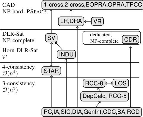
We now establish translations LC1 ! LC2 for calculi C1 and C2, briefly describing relations defined in the calculi to explain the constructions. Translations presented here have been selected to represent the four categories of Table 1. Results achieved are depicted graphically in Fig. 3 and further discussed in the next section. Any translation shown in the figure but not described in the following can be realized as a reduction among calculi and is described in the literature referenced in Table 1 for the respective calculus. To obtain connections that are not only reductions from some SAT(LC1 ) to some SAT(LC2 ) but translations which allow a L1-model to be derived from the resulting LC2-formula, the following proof ideas are constructive in the sense that they simulate LC1 entities and relations using a LC2-formula. To this end, it is sufficient to consider atomic LC1-formulas.
3.1 Temporal Calculi
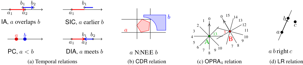
The following relationships are well-known (see respective references in Table 1 and illustrations in Fig. 1a) but repeated here for completeness. Interval relations of IA have been defined using atomic formulas of point-based PC constraints (thus IA ! PC), the converse direction directly follows from so-called 'pointizable' configurations in which intervals are not allowed to partially overlap and thus can represent points. Semi-interval relations in SIC are specified as disjunctions of IA relations, representing only the relative positions of the start points (respectively end points) of an interval. DIA extends the interval domain of IA by allowing intervals to point in either direction in time (rather 1-d space), hence refining IA relations to the relative orientation of intervals involved (same direction, head-on, departing). The additional expressivity can be simulated in IA by means of disjunctions ranging over the two possible orientations in 1-d, the other direction is obvious. INDU refines IA by introducing an additional comparison by relative length, therefore IA ! INDU holds.
3.2 Cardinal Direction Calculi
All translations among cardinal direction calculi shown in Fig. 3 directly follow from the respective literature given in Table 1, except for the following translation that achieves a connection from CDR to BA and equivalent calculi.
BA is a generalization of IA to two dimensions obtained by considering the projections of regions on the x- and y-axis as intervals and applying IA to these, i.e., BA relations are pairs of IA relations. Equivalence of IA and BA with respect to translations is thus obvious.
CDR is an expressive calculus related to BA for describing the location of simple regions in 2-d using cardinal directions. Two variants of CDR have been considered: one restricted to simple regions and one adressing regions not necessarily connected. Relations in CDR list the cardinal direction relations using an 8-sector model plus proximity zone, in which one region is located with respect to another, see Fig. 1b. This leads to 29 atomic relations in case of unconnected regions and 218 in case of connected regions [Liu et al., 2010]. Translations for the case of unconnected regions are straightforward by instantiating one box in BA for every sector mentioned in a CDR relation, so we focus on the case of connected regions.
Proposition 4. CDR!BA
Proof sketch. Construction follows the algorithm described in Liu et al. [2010]. Their algorithm constructs a canonical solution by joining a set of rectangular regions represented as pixels on a bitmap of size 2n ⇥ 2n for n entities. Here we use BA entities, which are boxes. For each base relation in a CSP(CDR) we introduce a chain of BA entities and enforce each box in the chain to be connected to its successor by means of BA relations (meets↪ ⇤) or (⇤↪meets) where ⇤ denotes the disjunction of all IA base relations. CDR base relations define a sequence of cardinal direction relations, e.g., N:NE:E as shown in Fig. 1b. We thus enforce the chain to follow these relations by restricting the ith element to the ith cardinal direction cell. It remains to be ensured that chains constructed for two different constraints but corresponding to the same CDR entity do not overlap with any direction not allowed by the CDR relations and that pairs of chains are connected, i.e., there exists an element in one overlapping an element in the other.
3.3 Relative Direction Calculi
OPRAm relates two oriented points with respect to their relative orientation towards each other [Mossakowski and Moratz, 2012], see Fig. 1c. An oriented point O is given by its Cartesian coordinates xO↪ yO 2 R and direction φO 2 [0↪ 2⇡] with respect to an absolute reference direction. OPRAm calculus is suited for representation of objects that have an intrinsic front or move in a particular direction and can be abstracted as points. Relations in OPRAm are sectors and linear relations equally dividing the full circle into 2m planar and 2m linear regions.
STARm is similar to OPRAm, except for the fact that all objects have the same directions (e.g., north). This has the effect that CSPSAT(STARm) is in P while OPRAm like almost any other directional calculus is NP-hard [Wolter and Lee, 2010]. Since we can construct basic axes using linear relations of OPRAm objects and force the directions of all other variables to be aligned with the one of the grid axes, we have that
Proposition 5. STARm !OPRAm.
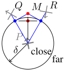
EOPRAm augments OPRAm with distance constraints, retaining the same set of directional relations. Each entity in EOPRAm has its own fixed threshold value δ for determining the qualitative distance (e.g., close and far) to other objects. Thus the entities in EOPRAm are defined as tuples (x↪ y↪ ✓↪ δ) 2 R2 ⇥ [0↪ 2⇡) ⇥R+0 . An example of the distance constraint is illustrated in Fig. 2a. Distance constraints can however easily be simulated in OPRAm, thus we have that
Proposition 6. OPRAm $EOPRAm.
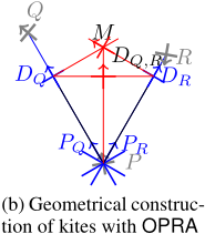
Proof sketch. Fig. 2a shows how a distance constraint of an EOPRAm object P with respect to another EOPRAm object Q can be emulated with the help of several dummy OPRAm objects to construct a kite. The construction detailed in Fig. 2b is possible since EOPRAm defines linear direction relations and superposition of objects with individual orientations. Two pairs of sides are of equal lengths in a kite. Its construction allows us to enforce that DQ and DR are in the same distance to P . Hence, by relating Q to DQ (respectively R to DR) we can compare their distance to a specific distance class δ associated with P .
3.4 Occlusion Calculi
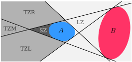
VR [Tarquini et al., 2007] describes locations of convex regions in the plane with respect to visibility relations. VR employs the partition scheme depicted in Fig. 2c, distinguishing five basic classes of visibility. For example, a location p is said to be in the shadow zone (SZ) of region A with respect to region B, if every line segment connecting an interior point of B with p also coincides with an interior point of A. Visibility is thus considered to be a ternary concept. Visibility relations among regions are determined by the zones in which interior points of a region are located, for example a region may be partially overlapping SZ and LZ, the light zone determined by full visibility of the target object. Zones of partial visibility are called twilight zones and further distinguished by whether the left side (TZL), the middle (TZM), or the right size (TZR) is occluded for an imaginary observer located in the plane. By construction, all zones are derived from lines connecting tangent points of regions (see Fig. 2c). Visibility relations may be regarded as a generalization of cyclic ordering for extended objects as is also captured by the LR calculus.
LR [Scivos and Nebel, 2005] is a calculus representing ternary point configurations, see Fig. 1d for illustration. Most importantly, LR defines the relations left and right: a b left c holds iff c is positioned on the left-hand side of the straight line -!ab, and a b right c iff c is positioned on the right-hand side of -!ab. Additional relations defined for the case when a↪ b↪ c are collinear are not relevant to establish the following construction:
Proposition 7. VR! LR.
- tion of kites with OPRA (c) Partitioning scheme with respect to regions A and B.
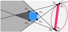
Figure 2: EOPRAm and VR
Proof sketch. We first note that it suffices to consider the set of convex polygons as the domain of VR instead of the set of convex 2D regions, because only a finite number of extreme points of each region affects visibility (see Fig. 2d). More specifically, those extreme points of a convex region are determined by four tangent lines induced by this region and another region. Therefore, in a scene with n regions, a region can be represented by its m := 4(n - 1) tangent points and we have altogether m · n points that determine a scene.
VR relations are ternary and we write AB RC to state that region C is located in region R 2 ¶TZL↪ TZM↪ TZR↪ SZ↪ LZ♦ of A with respect to object B. Now we show the translation of a VR-term AB SZC into an LR-formula. Other VRterms can be translated analogously. Note that since each VR variable is a polygon with m vertices, we can identify variables A↪B↪C with sequences of their vertices: A := (a1↪ ▷ ▷ ▷ ↪ am)↪B := (b1↪ ▷ ▷ ▷ ↪ bm)↪C := (c1↪ ▷ ▷ ▷ ↪ cm). For the resulting LR-formula we introduce quantifiers 8 and 9 for convenience; they can be replaced with V and W, respectively.AB SZ C
The explanation of the formula is as follows. In line (1) we impose convexity on the polygons, where
Then we specify four pairs (ai1 ↪ bj1 )↪ ▷ ▷ ▷ ↪ (ai4 ↪ bj4 ) of vertices of A and B that respectively determine the four tangent lines. In the case of the upper tangent from A to B the corresponding vertex pair (ai1 ↪ bj1 ) is specified by imposing that all vertices ai 2 A with ai 6= ai1 and all vertices bi 2 B with bi 6= bi1 are on the right-hand side of the directed line ---! ai1 bj1 (in Fig. 2d the upper tangent is the directed line --! a1b1). This specification is given in (2)-(4); here, Tangent1 determines the vertex pair for the upper tangent from A to B:
The definitions for Tangent2 ↪ Tangent3 ↪ Tangent4 can be obtained by changing the combination of the two LR-relations (right, right) occurring in the definition of Tangent1 to combinations (right, left), (left, right), (left, left), respectively.
Finally, in (5)-(7) we specify the location of C by stating that it is inside the polygon induced by the four tangent lines ---! ai1 bj1 ↪ ▷ ▷ ▷ ↪ ---! ai4 bj4 . Note that in (7) we impose that first, C does not overlap A, and second, C is behind A. The first condition is satisfied, if each vertex ci of C is outside A:
and the second condition is satisfied, if, in addition to the first condition, each vertex of C is to the right of directed line ---! ai1 ai4 (in Fig. 2d it is --! a1a2).
Line-Of-Sight Calculus (LOS) The Line-Of-Sight (LOS) calculus addresses the representation of occlusion from an observer-centered point of view. Entities in the calculus are regions in an observer's visual plane that result from the observation of physical objects and are thus assumed to be connected. Unlike RCC-8, regions in LOS cannot overlap but they are staggered in layers according to distance to the observer. LOS can be seen as a refined interpretation of RCC8 relations in which all modes of overlap, i.e., PO, TPP(i), NTPP(i), and EQ need to distinguish which region is in front of the other. This leads to an increased set of 14 atomic relations (LOS does not define an additional equality relation, but replaces RCC-8's EQ with the pair exactly hides/ exactly hidden by).
Proposition 8. LOS$RCC-8
Proof sketch. Technically speaking, LOS augments RCC-8 by a (depth) order for non-discrete entities. Assume topological information present in LOS to be represented using RCC8. To achieve LOS expressive power we additionally need to simulate its depth ordering: introduce a fresh depth variable DXi for every variable Xi and for every LOS constraint stating Xi to be in front of some Xj introduce the RCC-8 ordering constraint (DXi NTPP↪DXj ), and, analogously, using NTPPi in case Xi is behind Xj. This procedure is sufficient since LOS does not define equality, i.e., one cannot enforce two regions to be at the same distance to the observer.
4 Summary and Conclusion
This paper considers propositional closure of qualitative calculi as means for representing spatial (or temporal) knowledge. The main motivations of studying Boolean combinations of constraints is that they allow several interesting translations to be defined which cannot be exploited within the framework of qualitative calculi due to a lack of expressivity.
The main result of this paper is summarized in Fig. 3 which depicts individual calculi C arranged according to the reasoning algorithm required to solve SAT(LC) for atomic formulas. The vertical arrangement in layers separated by dashed lines also reflects the computational complexity with harder languages arranged towards the top. The following basic reasoning algorithms are involved:
- ÷ enforcing 3- and 4-consistency;
- ÷ solving Disjunctive Linear Programs (DLP), both their tractable Horn subclass (e.g., using algorithms presented in [Koubarakis, 2001] or [Jonsson and B¨ackstr¨om, 1998]) as well as the general case (e.g., by mixed integer linear programming solvers to encode disjunctions using integers);
- ÷ solving multivariate polynomial equations and inequalities (e.g., using Cylindrical Algebraic Decomposition (CAD) [Collins, 1974]).
By arrows we depict known translations, in case of mutual translations we group all calculi in a cluster. Clearly, translations are transitive but the figure only presents direct links to avoid visual clutter.
The translations depicted in Fig. 3 are important for two reasons: First, translations enable statements to be mixed that were originally composed using relations from two distinct calculi. This allows for joint reasoning which is important for practical applications, since qualitative calculi are highly specialized to a certain aspect of a single domain, but many tasks require several aspects (e.g., cardinal relations and visibility information) to be considered at once. To foster practical relevance we only consider translations that allow models obtained in the target languages to be mapped back.
Second, by translating one representation into another we are able to apply the same decision procedure to problem formulations originally given in two different qualitative formalisms, requiring two distinct techniques. This is useful for developers of versatile reasoning tools who wish to handle a wide range of spatial or temporal relations. The ability to translate one calculus into another language using Boolean combinations suggests a new approach in qualitative reasoning: to consider frameworks like SMT (see [Barrett et al., 2008] for an overview) or ASP [Lifschitz, 2008] with solvers supporting external theories, since both offer sophisticated means to address the propositional combinations occurring. Even if the translations lead to a higher class of complexity, the resulting method may be very efficient. While Westphal and W¨olfl [2009] have shown that highly optimized QSTR search techniques outperform SAT encodings in case of calculi with few relations (e.g., IA, RCC-8), they also discovered that SAT techniques become superior for calculi defining many atomic relations (e.g., CDR). SMT- or ASP-like techniques supporting specialized domain level reasoning are necessary since SAT is not sufficient to encode calculi from the CAD class which is conjectured to be beyond NP.
Acknowledgments
We gratefully acknowledge constructive comments by the anonymous reviewers. Diedrich Wolter acknowledges financial support by Technologieallianz Oberfranken. Jae Hee Lee acknowledges financial support by the Alexander von Humboldt foundation.
@inproceedings{ijcai2016p189,
  title     = {Connecting Qualitative Spatial and Temporal Representations by Propositional Closure},
  author    = {Wolter, Diedrich and Lee, Jae Hee},
  booktitle = {Proceedings of the Twenty-Fifth International Joint Conference on
               Artificial Intelligence, {IJCAI-16}},
  publisher = {AAAI Press / International Joint Conferences on Artificial Intelligence},
  editor    = {Subbarao Kambhampati},
  pages     = {1308--1313},
  year      = {2016},
  month     = {7},
  url       = {https://ijcai.org/proceedings/2016/189},
}
TY - CPAPER TI - Connecting Qualitative Spatial and Temporal Representations by Propositional Closure AU - Wolter, Diedrich AU - Lee, Jae Hee T2 - Proceedings of the Twenty-Fifth International Joint Conference on Artificial Intelligence, IJCAI-16 PB - AAAI Press / International Joint Conferences on Artificial Intelligence PY - 2016 SP - 1308 EP - 1313 UR - https://ijcai.org/proceedings/2016/189 ER -Copied
Machine-readable versions of this paper, for tools and AI agents:





