On Combinations of Binary Qualitative Constraint Calculi

1 Introduction

Qualitative constraint calculi are representation formalisms that allow for efficient reasoning about continuous (spatial or temporal) aspects of the world. The idea in Qualitative Spatial and Temporal Reasoning (QSTR) is to develop algorithmic techniques to reason about qualitative spatial and temporal relations: such relations abstract from concrete metrical data of entities (for example, time points, coordinate positions, distances) by subsuming similar configurations of entities into one qualitative representation.

Combinations of such calculi are of interest for several reasons. First, one can define new formalisms in which one can represent, and reason about, different aspects of a domain at the same time. Hence, combinations can be applied to increase the expressiveness of the formal language used to represent object configurations in the domain at hand. Second, representing relations as combinations of other relations sometimes allows for decomposing the relations between entities of a given domain into simpler relations. Finally, from a more practical point of view, combinations play an important role when qualitative spatial or temporal information, possibly from different sources, needs to be integrated and processed by exploiting semantic interdependencies between different relational schemata. For example, knowing the relative sizes between objects will already restrict the topological relations that are possible between these objects, and vice versa.

In fact, many calculi discussed in QSTR can be represented as combinations of other, simpler and more compact formalisms. For example, the cardinal direction calculus [Frank, 1996; Ligozat, 1998] can be defined as a specific twofold product of the point algebra [Vilain et al., 1989] and the rectangle algebra [Balbiani et al., 1998] is a twofold product of the interval algebra [Allen, 1983]. Contrary to such orthogonal combinations, combinations are more challenging in case that the relations considered in the calculi show semantic interdependencies. Typical examples of this kind of combination include the region occlusion calculus [Randell and Witkowski, 2002] as well as the combination of RCC-8 and the point algebra [Gerevini and Renz, 2002; Renz and Nebel, 2007].

With regard to non-orthogonal combinations, there exist two different possible combination strategies. Gerevini and Renz [2002] proposed a method for integrating such formalisms in a loose way by considering constraint networks in which edges can be labeled by pairs of relations, each of which stemming from one of the component calculi (e.g., each edge is labeled by both a topological relation and a qualitative size relation). For reasoning with such constraint networks (following referred to as biconstraint networks), Gerevini and Renz also presented an adaption of the usual path consistency algorithm (see e.g. [Mackworth and Freuder, 1985]) called bipath consistency algorithm and showed that this algorithm decides satisfiability for a rather large class of biconstraint networks with topological and qualitative size relations.

The second strategy is to build a new constraint language, which in general leads to a more tight integration. While in the bipath consistency method semantic interdependencies are propagated in the reasoning process only, these interdependencies are here exploited to define a new set of base relations and a new composition table, which often can be more refined than the composition table that one obtains from some Cartesian product construction.

In this paper we will investigate and compare both methods in more detail. We will show that tight combinations are more expressive than loose combinations via the biconstraint approach. Then we will report on an empirical study in which we compared both methods on randomly generated test instances to which both methods can be applied. These results indicate that the method of building a new calculus is more advantageous than the biconstraint approach provided that the compared reasoning processes can employ the same optimization strategies (in particular, techniques for the precomputation of composition tables).

2 Formal Background

In what follows let D be a fixed non-empty set. A (binary) relation system Γ over D is any non-empty set of binary relations on D. Given a relation system Γ, a constraint network over Γ is defined by a triple N = 〈V,D,C〉, where V is a finite set of variables, D is a non-empty set of values for the variables in V , and C is a finite set of constraints, i.e., pairs (s,R), where s = (x, y) is a pair of variables and R is one of the relations in Γ. If Γ is closed under intersection of relations and converse relations (i.e., R-1 := {(y, x) : (x, y) ∈ R} ∈ Γ for R ∈ Γ), one can assume that N contains for any pair of variables x, y at most one constraint with scope s = (x, y).

An assignment for a constraint network 〈V,D,C〉 is a function α : V → D. It is said to be a solution if for each constraint ((x, y),R) in C, (α(x), α(y)) ∈ R. A constraint network is said to be satisfiable if it has a solution.

Definition 1 ([Ligozat and Renz, 2004]). A partition scheme on a domain D is a finite binary relation system on D, Γ, that (a) forms a partition of D×D, (b) contains the identity relation {(x, x) : x ∈ D}, and (c) is closed under converses. The elements of Γ are usually referred to as the base relations of the partition scheme.

Given a partition scheme Γ, one usually considers constraint networks that allow for disjunctions of base relations (in order to represent imprecise information). Let Γ∗ denote the relation system consisting of all possible unions of relations from Γ (in contrast to base relations, the elements of Γ∗ are sometimes referred to as general relations).

Contrary to finite constraint networks, constraint networks in QSTR are defined on infinite domains. This entails that typical reasoning techniques known from the CSP domain (such as arc-consistency or path-consistency) are not directly applicable. Hence, the idea in QSTR is to restate constraint satisfaction problems on a symbolic level such that reasoning about specific variable assignments can be replaced by manipulation of symbol sets representing unions of concrete base relations.

Definition 2. A (binary) qualitative calculus is defined by a 4-tuple C = 〈B, ⌣ , ⋄, id〉, where B is a non-empty finite set of symbols (elements of B are also referred to as base relations), ⌣ : B → B is a unary function that assigns to each base relation its converse, ⋄ : B×B → 2B is a binary function that assigns to each pair of base relations their composition, and a distinguished element id ∈ B (the identity relation). We furthermore require that for a, b, c ∈ B, (a) (a⌣ )⌣ = a, (b) id ⋄ a = a⋄ id = a, (c) (a⋄ b)⌣ = b⌣ ⋄ a⌣ , (d) a⌣ ∈ b⋄ c iff c⌣ ∈ a ⋄ b.

Given a qualitative calculus in this sense, we have in a natural way a Boolean algebra on the set 2B (its elements are also referred to as general relations), and we obtain a nonassociative relation algebra if we extend the functions ⌣ and ⋄ to functions ⌣ : 2B → 2B and ⋄ : 2B × 2B → 2B , respectively, by: r⌣ := {b⌣ : b ∈ r} and r ⋄ r′ := ⋃b∈r,b′∈r′ b ⋄ b′ .

Let Γ be a partition scheme on D and let (bi)i∈I be a list of symbols, exactly one symbol b for each concrete relation bD ∈ Γ. The qualitative calculus associated to Γ, C[Γ], is defined as follows: B := {bi : i ∈ I}; id := bi, where bDi is the concrete identity relation on D; b⌣i := bj, where bDj is the concrete converse relation of bDi ; and

It is clear from the definition that in general the symbolic composition ⋄ is just an upper approximation of the settheoretical composition of concrete relations, that is, it holds:

If we can strengthen here the subset relation to equality, symbolic composition ⋄ is said to be strong (with respect to the partition scheme Γ), otherwise it is called weak.

Given a qualitative calculus C = 〈B, ⌣ , ⋄, id〉 associated to a partition scheme Γ, we can represent relations as sets of base relation symbols. In particular, constraints in a qualitative constraint network can be written in the form 〈(x, y), {b1, . . . , bk}〉 for relations bD1 , . . . , bDk ∈ Γ. Moreover, each constraint network N = 〈V,D, C〉 defines a constraint graph G = 〈V, l〉 such that V is just the set of variables of N and l : V × V → 2B is the function that assigns to each constraint scope (x, y) the symbol set {b1, . . . , bk}, where bD1 ∪ · · · ∪ bDk is the constraint relation between x and y. If there is no constraint with scope (x, y) in N, l assigns to (x, y) the set B of all relation symbols (which denotes the universal binary relation on D). A solution of a constraint graph G = 〈V, l〉, then, is a function α : V → D such that for all x, y ∈ V , (α(x), α(y)) ∈ bD for some b ∈ l(x, y).

A constraint graph 〈V, l〉 is said to be path-consistent (or: algebraically closed) if (a) no label is empty and (b) l(x, y) ⊆ l(x, z) ⋄ l(z, y) for each triple of variables x, y, z in V . Note that this notion is weaker than the notion of path consistency known from the CSP domain, which requires that each twovariable assignment that is consistent with the constraint network is extendable to a consistent three-variable assignment.

A constraint graph 〈V, l〉 is said to be a refinement of a constraint graph 〈V, l′ 〉 if l(x, y) ⊆ l′ (x, y) for each pair of variables from V . Each constraint graph can be refined (in polynomial time) into a constraint graph which is pathconsistent or inconsistent (that is, it has empty labels). This can be achieved if each of the labels l(x, y) (for variables x and y) is successively refined by applying the operation

where z is any third variable occurring in the network. Implementations of this method are usually based on one of the variants of Mackworth's path consistency algorithm [Mackworth and Freuder, 1985], which uses queues to store those arcs or triangles in the network that need to be re-processed due to previous refinements of the network.

Definition 3. Let C = 〈B, ⌣ , ⋄, id〉 be a qualitative calculus for a partition scheme Γ. A subset S of 2B is said to be a tractable subclass if the path consistency method applied to constraint graphs in which only relations from S occur decides satisfiability.

If the path consistency method decides satisfiability of atomic constraint graphs (a constraint graph is atomic if all its labels are singleton sets), then a constraint graph over 2B is satisfiable if and only if it has a path-consistent atomic refinement. By using backtracking methods, one can systematically check each atomic refinement of a given constraint graph for satisfiability (see, e.g., [Allen, 1983; Ladkin and Reinefeld, 1997]). Moreover, using tractable subclasses speeds up the reasoning time: instead of splitting a constraint during backtracking into base relations, it can be split into relations belonging to a tractable subclass. This leads to a considerable reduction of the branching factor of the search tree [Nebel, 1996].

3 CombinationMethods

In what follows, we will present two different methods for combining two constraint formalisms. We start by presenting a method that uses a kind of Cartesian product construction to form a new constraint calculus from two component calculi.

3.1 Tight Combination

For relation systems Γ1 and Γ2 on the same domain D, we define:

Lemma 1. If Γ1 and Γ2 are partition schemes on D, then so is Γ1 ⊗ Γ2.

Γ1⊗Γ2 obviously provides a partition of D×D, it contains the identity relation, and it is closed under converses (note that (R1 ∩ R2)-1 = R-1 1 ∩R-1 2 ).

In what follows let Γ1 and Γ2 be partition schemes defined on D. Since Γ1 ⊗ Γ2 is a partition scheme, it defines an associated constraint calculus C[Γ1 ⊗Γ2]. On the other hand, we have constraint calculi C[Γ1] and C[Γ2] associated to Γ1 and Γ2, respectively. How are they related? For this, we first need to fix the interdependencies between Γ1 and Γ2 on the symbolic level. We define a function IΓ1,Γ2 :BΓ1 → 2BΓ2 which maps a base relation b of BΓ1 to the set of those base relations of BΓ2 that have a non-empty intersection with b, if interpreted over D, i.e., bD ∩ b′D ̸= ∅ for all b′ ∈ IΓ1,Γ2 (b). Note that b′ ∈ IΓ1,Γ2 (b) iff b ∈ IΓ2,Γ1 (b′ ).

Definition 4. Given constraint calculi C1 = 〈B1, ⌣1 , ⋄1, id1 〉 and C2 = 〈B2, ⌣2 , ⋄2, id2 〉 and an interdependency function I1,2 :B1 → 2B2 , the product constraint calculus C1 ⊗ C2 is defined as follows:

The interpretation of a general relation r of C[Γ1] ⊗ C[Γ2] is just rD := ⋃(b1,b2)∈r bD1 ∩ bD2 . Note that there is also a function that maps each base relation b of C[Γ1 ⊗ Γ2] to a "base relation" of C[Γ1] ⊗ C[Γ2], namely the pair of base relations ˆb := (b1, b2) such that bD1 ∈ Γ1, bD2 ∈ Γ2, and bD = bD1 ∩bD2 . Hence each set r of base relations of C[Γ1⊗Γ2] can be identified with a set ˆ r of base relations of C[Γ1] ⊗C[Γ2] as well.

Let C1 and C2 be qualitative calculi with the same set of base relations and the same converse mapping. C1 is said to be compositionally at least as fine as C2 if for all base relations b, b′ , it holds b ⋄1 b′ ⊆ b ⋄2 b′ .

Theorem 1. Given the partition schemes Γ1 and Γ2 as before, C[Γ1 ⊗Γ2] defines a qualitative calculus that is compositionally at least as fine as C[Γ1]⊗C[Γ2] if the base relations of C[Γ1 ⊗ Γ2] are identified with pairs of base relations of C[Γ1] ⊗ C[Γ2].

We can also transfer tractability results from the component calculi to the combined calculus. For this consider subclasses S1 and S2 of C[Γ1] and C[Γ2], respectively. Let S1 ⊗S2 denote the set of general relations r of C[Γ1]⊗C[Γ2] such that there exist r1 ∈ S1 and r2 ∈ S2 with rD = rD 1 ∩rD 2 . Then each constraint graph G = 〈V, l〉 with labels from S1 ⊗ S2 can be decomposed into two constraint graphs with the same set of variables, the first, G|S1 , with labels from S1 and the second, G|S2 , with labels from S2.

Theorem 2. Let C[Γ1] and C[Γ2] be qualitative calculi associated to Γ1 and Γ2, respectively. If S1 and S2 are tractable subclasses of C[Γ1] and C[Γ2], resp., such that each constraint graph G with labels from S1 ⊗ S2 is satisfiable if both G|S1 and G|S2 are satisfiable, then S1 ⊗S2 is a tractable subclass of C[Γ1] ⊗ C[Γ2].

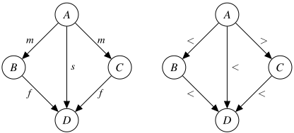
This theorem states that if a constraint network over C[Γ1] ⊗ C[Γ2] can be decomposed into two constraint networks, each with relations from a tractable subclass, and if solutions of these networks can be glued together in a consistent way (a counterexample is given in Figure 1), then this network can also be decided by the path consistency method.

3.2 Loose Combination

Definition 5. Let Γ1 and Γ2 be partition schemes. A biconstraint network over Γ1 and Γ2 is a constraint network over (Γ∗1 ⊗Γ∗2 )∪{∅}. Alternatively, if we allowmore than one constraint for each constraint scope, biconstraint networks can be defined as constraint networks over Γ∗1 ∪ Γ∗2 .

Biconstraint networks can be expressed on the symbolic level by pairs of constraint networks on the same set of variables. To put this more formally, let C1 = 〈B1, ⌣1 , ⋄1, id1 〉

and C2 = 〈B2, ⌣2 , ⋄2, id2 〉 be constraint calculi with interdependency function I1,2 : B1 → 2B2 . The function I1,2 can be lifted to a function ˆ I1,2 : 2B1 → 2B2 if we set ˆ I1,2(r) := ⋃b∈r I1,2(b). Then, a biconstraint graph is a triple G = 〈V, l1, l2〉 where V is a set of variables and the li : V 2 → 2Bi are labeling functions as in the case of ordinary constraint networks. That is, a biconstraint graph labels each edge with a pair of general relations (l1(x, y)), l2(x, y)) ∈ 2B1 × 2B2 .

To decide consistency of biconstraint networks, Gerevini and Renz [2002] propose the O(n3 )-time bipath consistency algorithm, which is an adaption of the path consistency algorithm. Bipath consistency enforces path consistency to both parts of a biconstraint network in parallel and propagates information between the two part networks using the interdependency function. Hence, all operations on relations are performed separately in the two calculi except for the propagation of interdependency constraints. The algorithm uses a birevision function that plays a role analogous to the revision function (1) used in the usual path consistency algorithm. Moreover, similar to path consistency, tractable subclasses exist and we can use backtracking search for deciding satisfiability if the used base relations are tractable.

Note, that we can assign to each loose combination a tight one via the induced product constraint calculus. Thus, any biconstraint network can be written as a constraint network over the tight combination, but not vice versa (cf. next section). Specifically, the revision function (1) applied to networks in the product calculus is at least as strong as the birevision function. This also allows for translating tractability results for the loose combination to the tight combination.

We conclude the section with the following definition: A combination method of constraint calculi C1 and C2 with interdependency map I1,2 is said to be orthogonal if I1,2(b) = B2 for each b ∈ B1.

4 Examples

Following we briefly sketch some combination representations of calculi that are well known in the literature. We start with two examples of orthogonal combinations.

Example 1 (Cardinal directions calculus [Ligozat, 1998]). Consider points in the Euclidean plane R2 as the underlying domain and define the base relations of the cardinal direction calculus as pairs of point algebra relations (e.g., [Vilain et al., 1989]), i.e., one compares the x- and y-coordinates of two points in the plane. Thus, the orthogonal product of the point algebra with itself yields the cardinal directions calculus.

Example 2 (Rectangle algebra [Balbiani et al., 1998]). Consider rectangles in the Euclidean plane, where each side of the rectangles is parallel to the x- or to the y-axis. As base relations consider pairs of base relations of Allen's interval algebra, which describe the Allen relation between the projection of two rectangles to the x- and the y-axis, respectively. Thus, the rectangle algebra is the 2-fold orthogonal product of Allen's interval algebra.

Example 3 (Allen's interval algebra [Allen, 1983]). Consider the reals as time line and as domain the set of Allen intervals (t, t′ ) ∈ R2 with t < t′ . We can define the base relations of the interval algebra as 4-tuples of base relations of the point algebra if we compare the start and endpoint of two intervals, respectively. This combination is not orthogonal. For example, if the endpoint of an interval precedes the start point of another interval, it also precedes the endpoint of the second interval.

Example 4 (The interval duration network calculus (INDU) [Pujari et al., 1999]). Consider Allen intervals in the real time line as in the previous example. We now compare Allen intervals not only in terms of the usual Allen interval relations, but also with respect to their size (length). Qualitative size information can be expressed by using point algebra relations. Again there exist semantic interdependencies, e.g., if two intervals are equal, then so is their size. Thus, the INDU calculus is a non-orthogonal combination of Allen's interval algebra and the point algebra. It should also be mentioned that the path consistency method does not decide satisfiability even if one just considers networks with base relations.

Example 5 (Closed disc algebra and cardinal directions calculus [Ragni and W¨olfl, 2008]). As domain consider the set of closed discs in the Euclidean plane R2 . We compare these discs with respect to topological relations (RCC-8) and the cardinal directions of the disc centers. In this formalism we have semantic interdependencies between both sets of base relations (e.g., if two closed discs are equal, so is their position). Note that the calculus resulting from composing the partition schemes is compositionally finer than the product of the considered component calculi. For example, it holds:

Example 6 (RCC-8 and qualitative size QS [Gerevini and Renz, 2002]). Gerevini and Renz proposed to combine the RCC-8 calculus with qualitative size information, i.e., point algebra relations. For this, consider as domain measurable sets of Rn , e.g., spheres. As mentioned previously, the authors represented spatial information as biconstraint networks. Obviously, this loose combination is not orthogonal. For example, if two regions are equal, so is their size.

Example 7 (RCC-8 and qualitative size QS ∗ ). Instead of representing RCC-8 with qualitative size information as biconstraint networks (i.e., loose combination), we form a new tight combination by building a calculus using the interdependencies presented in [Gerevini and Renz, 2002].

The difference in expressiveness between the (loose) biconstraint representation and the (tight) product method can be demonstrated if we revisit the last two examples.

As a general rule, with loose combinations one can only express relations that can be represented as pairs of complex relations of the component calculi. Hence, if we loosely combine two calculi with n1 and n2 base relations, respectively, we obtain a formalism which can express at most 2n1 · 2n2 different relations, possibly less when interdependencies are taken into account. In the case of tight combinations, all unions of pairs of base relations can be expressed, which results in up to 2n1·n2 different relations for orthogonal products.

For the combination of RCC-8 and QS, we obtain 549 distinct relations for the loose (Example 6), and 16384 relations for the tight combination (Example 7). In the formalism of Example 6, it is, for example, not possible to specify mixed indefinite knowledge such as:

Only an upper approximation

can be formalized.

Clearly, the tight combination is always more expressive than a loose one. However, for reasoning purposes this advantage can turn into a problem, since in general the search space for checking satisfiability of constraint networks increases considerably.

5 Comparing Tight and Loose Combinations Empirically

We compared the performance of reasoning with constraint networks combining RCC-8 and qualitative size information. To compare tight and loose combinations, we considered satisfiability tests of randomly generated constraint networks.

5.1 Problem Instances

Our method of generating problem instances is adapted from the one described in [Renz and Nebel, 2007]. To provide a fair comparison, we generated only constraint networks with constraint relations that have a Cartesian product form: hence both procedures received a semantically equivalent input. The instance generation method uses the parameters n (number of nodes) and d (average degree), and can be described as follows:

1. Generate a complete constraint graph with n nodes such that each is edge is labeled with the universal relation.
2. Pick n·d 2 edges at randomwith uniform distribution. For each such edge pick non-empty relations R ∈ C[Γ1] and S ∈ C[Γ2], each with a uniform distribution, and assign to the edge the relation R ∩ S. If R ∩ S = ∅, we pick these two relations randomly again.

We found that already for d = 2.25 instances with 100 nodes have a probability of around 50% for being consistent. Hence, we used as average degree d = 2 to generate all of the test instances independently of the actual network size.

5.2 Implementation and Test Environment

The bipath consistency method was implemented in the Generic Qualitative Reasoner (GQR) 1 [Gantner et al., 2008]. GQR already provides precomputation techniques for the composition function of general relations [Ladkin and Reinefeld, 1997], as used in the path consistency method. For the bipath consistency algorithm, the corresponding constraint propagation function requires the computation of the interdependency function (in addition to the ⋄-functions of RCC-8 and the point algebra). Also here we used precomputations of all these functions.

The benchmarks were run on an Intel Xeon processor with 3 GHz and 3 GiB of memory.

5.3 Empirical Results

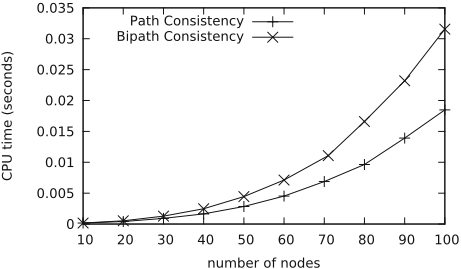
First, we compared the constraint propagation step, that is, the run-time of path consistency and bipath consistency. The results of this comparison (depicted in Figure 2) are based on full precomputations of the composition function of general relations. Our results indicate that the birevision function performs worse than the revision function, presumably due to the overhead that arises from the fact that all operations must be performed on two networks. However, one should keep in mind that precomputations of the composition function for general relations are infeasible for large calculi, since the resulting look-up tables grow exponentially in the number of base relations. Hence different results can be expected for combinations of large calculi, where the full precomputation is not possible.

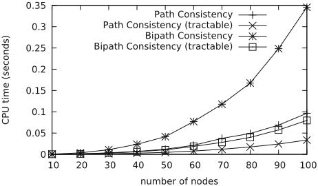
Second, we considered the entire reasoning process (see Figure 3). If no tractable subclasses are used, then reasoning with the backtracking algorithm in conjunction with path consistency turns out to be much faster than the backtracking algorithm using bipath consistency. We conjecture that this is due to the worse pruning achieved by bipath consistency and the overhead of the biconstraint approach, i.e., the maintenance of two constraint networks. If the tractable subclass ̂H8 × 2{<,=,>} (cf. [Gerevini and Renz, 2002]) is exploited, the performance difference decreases considerably, but is still observable. In general both approaches perform better when information about tractable subclasses is used.

1 http://sfbtr8.informatik.uni-freiburg.de/ R4LogoSpace/Resources/GQR

6 Conclusion

In this paper we considered different methods to combine qualitative constraint calculi from a general point of view. We formally defined methods for tight and loose combinations of such formalisms, and showed some relationships between these approaches.

For a particular combination (RCC-8 with qualitative size relations), we performed empirical tests on how reasoning based on the bipath consistency algorithm compares to reasoning using path consistency. From our empirical evaluation, it can be concluded that for certain combinations a tight integration approach is both feasible and even more efficient than a loose one. However, this result depends crucially on the size of the considered calculi and presumably also on tractability results. Moreover, in this paper we neglected heuristic search methods that could be used to improve the reasoning performance. Finally, it remains an open problem how other combinations such as the directed interval algebra [Renz and Nebel, 2007] can be represented in this framework.

Acknowledgments

This work was partially supported by Deutsche Forschungsgemeinschaft (DFG) as part of the Transregional Collaborative Research Center SFB/TR 8 Spatial Cognition (project R4[LogoSpace]).