
Increasingly Cautious Optimism for Practical PAC-MDP Exploration
Proceedings of the Twenty-Fourth International Joint Conference on Artificial Intelligence. Special Track on Machine Learning. Pages 4041-4047.
© 2015 International Joint Conferences on Artificial Intelligence
Abstract
Exploration strategy is an essential part of learning agents in model-based Reinforcement Learning. R-MAX and V-MAX are PAC-MDP strategies proved to have polynomial sample complexity; yet, their exploration behavior tend to be overly cautious in practice. We propose the principle of Increasingly Cautious Optimism (ICO) to automatically cut off unnecessarily cautious exploration, and apply ICO to R-MAX and V-MAX, yielding two new strategies, namely Increasingly Cautious R-MAX (ICR) and Increasingly Cautious V-MAX (ICV). We prove that both ICR and ICV are PACMDP, and show that their improvement is guaranteed by a tighter sample complexity upper bound. Then, we demonstrate their significantly improved performance through empirical results.
- [Brafman and Tennenholtz, 2002] Ronen I. Brafman and Moshe Tennenholtz. R-max-a general polynomial time al- gorithm for near-optimal reinforcement learning. Journal of Machine Learning Research, 3:213-231, 2002. IJCAI
- [Dearden et al., 1998] Richard Dearden, Nir Friedman, and Stuart J. Russell. Bayesian Q-learning. In Proceedings of the Fifteenth National Conference on Artificial Intelli- gence (AAAI-98), pages 761-768, 1998.
- [Kaelbling et al., 1996] Leslie P. Kaelbling, Michael L. Littman, and Andrew W. Moore. Reinforcement learn- ing: A survey. Journal of Artificial Intelligence Research, pages 237-285, 1996.
- [Kakade, 2003] Sham M. Kakade. On the sample complexity of reinforcement learning. PhD thesis, University College London, 2003.
- [Kolter and Ng, 2009] J. Zico Kolter and Andrew Y. Ng. Near-Bayesian exploration in polynomial time. In Pro- ceedings of the 26th International Conference on Machine Learning, pages 513-520, 2009.
- [Lattimore and Hutter, 2014] Tor Lattimore and Marcus Hutter. Near-optimal PAC bounds for discounted MDPs. Theoretical Computer Science, 558:125-143, 2014.
- [Leffler et al., 2007] Bethany R. Leffler, Michael L. Littman, and Timothy Edmunds. Efficient reinforcement learning with relocatable action models. In Proceedings of the 22nd National Conference on Artificial Intelligence -Volume 1, AAAI'07, pages 572-577. AAAI Press, 2007.
- [Li et al., 2011] Lihong Li, Michael L. Littman, Thomas J. Walsh, and Alexander L. Strehl. Knows what it knows: a framework for self-aware learning. Machine learning, 82(3):399-443, 2011.
- [Li, 2012] Lihong Li. Sample complexity bounds of ex- ploration. In Reinforcement Learning, pages 175-204. Springer, 2012.
- [Meuleau and Bourgine, 1999] Nicolas Meuleau and Paul Bourgine. Exploration of multi-state environments: Local measures and back-propagation of uncertainty. Machine Learning, 35(2):117-154, 1999.
- [Puterman, 1994] Martin Puterman. Markov Decision Processes: Discrete Stochastic Dynamic Programming. Wiley-Interscience, 1994.
- [Rao and Whiteson, 2012] Karun Rao and Shimon White- son. V-max: tempered optimism for better PAC rein- forcement learning. In Proceedings of the 11th Interna- tional Conference on Autonomous Agents and Multiagent Systems-Volume 1, pages 375-382, 2012.
- [Strehl and Littman, 2004] Alexander L. Strehl and Michael L. Littman. An empirical evaluation of in- terval estimation for markov decision processes. In Tools with Artificial Intelligence (ICTAI), 2004., pages 128-135, 2004.
- [Strehl and Littman, 2005] Alexander L. Strehl and Michael L. Littman. A theoretical analysis of model- based interval estimation. In Proceedings of the 22nd International Conference on Machine learning, pages 856-863. ACM, 2005.
- [Strehl et al., 2006] Alexander L Strehl, Lihong Li, Eric Wiewiora, John Langford, and Michael L Littman. PAC model-free reinforcement learning. In Proceedings of the 23rd International Conference on Machine learning, pages 881-888. ACM, 2006.
- [Strehl et al., 2009] Alexander L. Strehl, Lihong Li, and Michael L. Littman. Reinforcement learning in finite MDPs: PAC analysis. The Journal of Machine Learning Research, 10:2413-2444, 2009.
- [Sutton and Barto, 1998] Richard S. Sutton and Andrew G. Barto. Introduction to Reinforcement Learning. MIT Press, Cambridge, MA, USA, 1st edition, 1998.
- [Szita and Lőrincz, 2008] István Szita and András Lőrincz. The many faces of optimism: A unifying approach. In Proceedings of the 25th International Conference on Ma- chine Learning, pages 1048-1055, 2008.
- [Szita and Szepesvári, 2010] István Szita and Csaba Szepesvári. Model-based reinforcement learning with nearly tight exploration complexity bounds. In Proceed- ings of the 27th International Conference on Machine Learning, pages 1031-1038, 2010.
- [Whitehead, 1991] Steven D. Whitehead. Complexity and cooperation in Q-learning. In Proceedings of the Eighth International Workshop on Machine Learning, pages 363- 367, 1991.
- [Wiering and Schmidhuber, 1998] Marco Wiering and Jürgen Schmidhuber. Efficient model-based exploration. In Proceedings of the Fifth International Conference on Simulation of Adaptive Behavior (SAB98), pages 223-228, 1998.
References were extracted automatically from the PDF and may contain errors.
Full text extracted automatically from the PDF; figures, tables and equations may differ. The PDF is the version of record.
1 Introduction
In Reinforcement Learning (RL) [Sutton and Barto, 1998], exploration strategy is a key component of learning algorithms. By following an exploration strategy, the agent in model-based RL interacts with an initially unknown environment, often formulated as a Markov Decision Process (MDP), to collect information in the form of samples of the dynamics. The collected samples are used to build a model of the MDP, and the model is used to derive a policy that yields maximal expected cumulative rewards received from the environment. Simple undirected strategies such as ε-greedy could lead to exponentially inefficient exploration and poor performance [Whitehead, 1991; Li, 2012], and therefore, numerous strategies have been proposed and studied.
Efficiency of exploration strategies can be quantified and analyzed formally in the framework of sample complexity [Kakade, 2003] and Probably Approximately Correct in Markov Decision Process (PAC-MDP) [Strehl et al., 2009]. The sample complexity of an exploration strategy is the number of timesteps that the strategy, seen as a policy, is not nearoptimal in an infinite-length learning process. An exploration strategy is said to be PAC-MDP if it has a sample complexity bounded by some polynomial in the relevant quantities of the learning task with high probability. Various strategies have been proved to be PAC-MDP, such as R-MAX [Brafman and Tennenholtz, 2002], Model-Based Interval Estimation [Strehl and Littman, 2005], Delayed Q-Learning [Strehl et al., 2006], Optimistic Initial Model (OIM) [Szita and L˝orincz, 2008], MoRMAX [Szita and Szepesv´ari, 2010], V-MAX [Rao and Whiteson, 2012], and UCRLγ [Lattimore and Hutter, 2014].
∗Corresponding author.
One major drawback of most PAC-MDP strategies is that their exploration behavior can be overly cautious [Kolter and Ng, 2009]. Under these strategies, the agent is encouraged to sample every state-action pair repeatedly until the model is sure to be near-accurate. However, a near-accurate model is not always necessary for deriving a near-optimal policy [Kakade, 2003]. Consequently, existing PAC-MDP strategies may re-visit partly known state-action pairs too often, and miss the chance of discovering the near-optimal policy earlier. In practical use, this problem can be partially alleviated by manually setting the cautiousness to some insufficient degree compared to the degree required by the PAC-MDP theorems of these strategies. However, doing so actually removes the PAC-MDP property from the strategies and increases the risk of convergence to undesirable policies.
In this paper, we provide an effective solution to this dilemma by proposing the principle of Increasingly Cautious Optimism (ICO). The key idea of ICO is to set the initial cautiousness of optimistic exploration to extremely low, and gradually increase the cautiousness during the learning process. In this way, unnecessary exploration can be effectively reduced, leading to high practical efficiency, while the PACMDP property of the strategy is kept undamaged, avoiding any additional risk of undesirable convergence.
By applying the principle of ICO, we propose a modified version of R-MAX and V-MAX respectively, namely Increasingly Cautious R-MAX (ICR) and Increasingly Cautious VMAX (ICV). We prove that the existing sample complexity upper bound for R-MAX and V-MAX holds for ICR and ICV. Then, we derive a tighter upper bound for ICR and ICV under an additional assumption to show that their improvement is theoretically supported. Finally, we display their significantly improved practical performance through experiments.
2 Background
A finite MDP is a tuple (S, A, T, R, γ) that describes the dynamics of an environment, where S is a finite set of states, A is a finite set of actions, T : S × A × S ↦→[0, 1] is the transition probability to next states given current state and action, R : S × A × S ↦→R is the deterministic immediate reward for every possible transition, and γ ∈ [0, 1) is a discounted factor to future rewards. A policy π : S ↦→A instructs which action should be taken given the current state. A state-action value Qπ (s, a) is the expected discounted cumulative reward starting from the state-action pair (s, a) and following π afterwards; a state value V π (s) is the maximum of Qπ (s, a) with the same s. Without loss of generality, we assume R is bounded in [0, Rmax]; then it follows that the maximum possible state value Vmax is no larger than Rmax/(1γ). An optimal policy π∗ selects actions that yield best expected discounted cumulative rewards at any possible states, and its value functions are denoted by Q∗ and V ∗ . A more detailed introduction can be found in [Sutton and Barto, 1998].
In model-based reinforcement learning, the agent continuously interacts with the environment, and collects samples in the form of (s, a, s′ , r). The multiset of collected samples, denoted by ψ, is used to construct a model to estimate the dynamics of the MDP, and a policy π can be derived from the model using a planning algorithm. An exploration strategy σ : Ψ × S ↦→A maps a multiset of collected samples and a state to an action, where Ψ is the set of all possible ψ. The role of exploration strategies is to guide the agent during learning so that it could collect samples efficiently.
In this paper, we consider the common basic setting that the model is built using maximum likelihood estimation (MLE):
where nψ(s, a) and nψ(s, a, s′ ) stand for the numbers of corresponding transitions in the collected samples ψ, and rψ(s, a, s′ ) stands for the total reward obtained along with the transitions (subscript ψ will be omitted if no ambiguity occurs). For concreteness and convenience, we always use Value Iteration (VI) [Puterman, 1994; Sutton and Barto, 1998] as the planning algorithm in this paper. However, the results can be applied to other planning algorithms easily as long as they have some sufficient accuracy guarantee.
Sample complexity is a theoretical framework for analyzing efficiency of an exploration strategy. Given an arbitrary ε > 0, the sample complexity of a strategy σ is the number of timesteps that σ(ψt) seen as a policy is not ε-optimal at the current state, that is, V σ(ψt) (st) ≥ V ∗ (st) - ε does not hold, during the whole learning process [Kakade, 2003]. A strategy σ is said to be PAC-MDP if for any ε > 0 and 0 < δ < 1, the sample complexity of σ is bounded by some polynomial in the relevant quantities (|S|, |A|, Vmax, 1/ε, 1/δ, 1/(1 - γ)), with probability at least 1 - δ [Strehl et al., 2009].
R-MAX [Brafman and Tennenholtz, 2002] is a famous PAC-MDP exploration strategy based on the principle of optimism in the face of uncertainty [Kaelbling et al., 1996]. RMAX explicitly distinguishes known state-action pairs from unknown ones. Initially, all possible state-action pairs are marked as unknown; a state-action pair becomes known if it has been sampled at least m times, where m is a parameter of the strategy and needs to be set manually. The agent always chooses greedy actions at = argmaxa ˆQ(st, a) at every timestep t. Instead of a model built purely by MLE, here ˆQ is calculated from an optimistic model:
where sI is a fictitious absorbing state where the agent always receives rewards as large as (1 - γ)Vmax. By using Bellman Equation (see [Sutton and Barto, 1998]), it can be derived that ˆQ(s, a) = Vmax holds for all unknown (s, a); this forces the agent to explore unknown state-action pairs before re-visiting known ones. Additionally, any further samples gained for known state-action pairs will be discarded and not be used in the optimistic model, so that the total times of update is bounded. The upper bound on sample complexity ˜O( |S|2 |A|V 3 max ε3 (1-γ)3 ) holds for R-MAX with some m = ˜O( |S|V 2 max
The performance of R-MAX tends to be poor in practice due to its unbiased exploration among unknown stateaction pairs, no matter if they are promising or clearly nonpromising [Strehl and Littman, 2004]. To achieve better performance, V-MAX [Rao and Whiteson, 2012], a state-ofthe-art PAC-MDP strategy, encourages exploration to more promising unknown state-action pairs by biasing its optimism with experience. Specifically, the optimistic bonus is mixed linearly with the realistic MLE by a modified estimation:
so that the unknown state-action pairs with fewer samples and greater estimated values will be visited first. The upper bound on sample complexity for R-MAX ˜O( |S|2 |A|V 3 max ε3 (1-γ)3 ) holds for VMAX subject to the same condition of m.
3 Increasingly Cautious Optimism
The other face of the extreme optimism in R-MAX and VMAX is extreme cautiousness: the agent is forced to sample every state-action pair repeatedly unless it is convinced that the collected samples are sufficient to make a near-accurate estimate of the dynamics with high probability.
Unfortunately, this cautiousness is not always necessary. According to [Kakade, 2003], if a generative model for the MDP is available, which allows the agent to obtain samples of any state-action pairs at anytime, then the sample complexity is only linear to |S||A|. As the size of the full transition matrix is |S|2 |A|, this suggests that an ε-optimal policy can be derived from a very coarse model. Therefore, these overly cautious PAC-MDP exploration strategies can be far from efficient, in the sense that they aim to build up nearaccurate model from the beginning, and consequently miss the chance to find out ε-optimal policy earlier. This problem can be partly alleviated by carefully hand-tuning the cautiousness parameters of the strategies. However, doing so usually breaks the precondition of the PAC-MDP property, and may considerably increase the risk of early convergence to non-εoptimal policies [Strehl and Littman, 2004].
To solve this problem more effectively, we propose the principle of Increasingly Cautious Optimism (ICO). Specifically, an ICO strategy initially presume that the learning task is very easy, in the sense that an extremely careless optimistic exploration is sufficient to build a model which is accurate enough to be used to derive an ε-optimal policy. If the agent is lucky enough to find out an ε-optimal policy quickly, then the excessive sampling has already been reduced. Yet this initial exploration scheme might not be sufficient; to avoid convergence to undesirable policies, ICO increases the degree of cautious optimism over time, forcing the agent to sample every state-action pair gradually more often.
In this way, the agent explores with a much lower degree of cautiousness in general, reducing the possible overly cautious sampling encouraged by the original strategies. Meanwhile, the PAC-MDP property is still undamaged, as the degree of cautiousness eventually grows to the level required by the original theorems in bounded timesteps.
3.1 Increasingly Cautious R-MAX (ICR)
By applying the principle of ICO to R-MAX, we invent the novel exploration strategy of Increasingly Cautious R-MAX (ICR). We denote the original fixed m of R-MAX as mmax, and introduce a positive real number mt ≤ mmax to represent the current cautiousness of optimistic exploration. The mt increases linearly with a fixed real number Δm > 0 along with timestep t. Naturally, m0 corresponds to the initial careless setting. The optimistic modeling in R-MAX is altered by replacing the original fixed m with the increasing ⌊mt⌋:
The resulting pseudo-code for ICR is given in Algorithm 1.
Algorithm 1 Increasingly Cautious R-MAX(m0, Δm, mmax)
- 1: Multiset of collected samples ψ ← ∅
˜
- 2: Initialize T , ˜R using Equation 6, 4
- 3: ˜Q(s, a) ← Vmax for all (s, a)
- 4: for timestep t = 1, 2, 3, ... do
- 5: Observe current state st
- 6: Execute greedy action at ← argmaxa ˜Q(st, a)
- 7: Receive reward rt and transit to the next state st+1
- 8: ψ ←ψ ∪ (st, at, st+1, rt)
- 9: mt ←min(mt-1 +Δm,mmax)
- 10: if ⌊mt⌋ > ⌊mt-1⌋ then
˜
- 11: Update T for all (s, a) that n(s, a) < ⌊mt⌋ using Equation 6
- 12: if ⌊mt⌋ ≤ n(st, at) ≤ mmax then
˜
- 13: Update T (st, at, ·), ˜R(st, at, ·) using Equation 6, 4
˜
- 14: Update ˜Q by VI if T has been updated
We focus on the new mechanisms of ICR in this part; the parameter setting for m0, Δm, and mmax will be discussed in Section 3.2. Each time line 14 finishes, every (s, a) falls into one of the three exclusive status: unknown (n(s, a) < ⌊mt⌋), known-for-now (⌊mt⌋ ≤ n(s, a) < mmax), and known (n(s, a) ≥ mmax), named after the manners in R-MAX.
All unknown (s, a) have a value of Vmax and will be optimistically explored by the agent as in R-MAX. However, as soon as the (s, a) turns into known-for-now, the optimistic ˜ T , ˜R and ˜Q will be replaced by their realistic estimates based on the collected samples ψ in line 12-14. This leads to a relatively careless sampling scheme, which may increase the risk of convergence to non-ε-optimal policies.
Fortunately, any possible premature convergence will be corrected by ICR, as known-for-now (s, a) will turn back to unknown when the increasing ⌊mt⌋ exceeds n(s, a). To regain optimism, a re-optimisticalization operation, which overwrite realistic estimates again by the optimistic ones, will be performed on these newly unknown (s, a) as in line 10-11. This will not lead to a loss in collected information, since all the samples are kept in ψ for future use.
Finally, all (s, a) will eventually become known; after that, they are treated exactly as in R-MAX, where all further collected samples will be ignored.
3.2 Sample Complexity Analysis for ICR
First, we prove that the existing sample complexity upper bound for R-MAX holds for ICR. We then introduce the concept of relaxed tasks, and use the first bound to derive a tighter upper bound for ICR under an additional assumption.
Theorem 3.1. Given arbitrary MDP M = (S, A, T, R, γ), ε > 0, and 0 < δ < 1, there exists mmax = ˜O( |S|V 2 max ε2 (1-γ)2 ), such that for all (m0, Δm) satisfying 1 ≤ m0 ≤ mmax and mmax-m0 Δm = ˜O( |S|2 |A|V 3 max ε3 (1-γ)3 ), the following holds. If ICR is executed on M with parameter (m0, Δm,mmax), then with probability at least 1 - δ, the sample complexity of ICR is bounded by ˜O( |S|2 |A|V 3 max ε3 (1-γ)3 ).
Proof. (sketch) As m0 ≤ mmax and Δm > 0, ICR can be seen as a two-stage algorithm: mt < mmax, and mt = mmax.
In the most agnostic situation, ICR is non-ε-optimal in all steps before mt reaches mmax, resulting in an additional overhead to the sample complexity. Under the parameter setting for ICR in Theorem 3.1, this additional overhead of the first
˜O( |S|2 |A|V 3 ε3 (1-γ)3 ) steps.
Then, ICR starts behaving exactly as an R-MAX with parameter m = mmax, except that it has already collected mmax-m0 Δm samples. In the proof of sample complexity upper bound of R-MAX in [Strehl et al., 2009], it is irrelevant whether the R-MAX starts with a non-empty multiset of samples or not, as long as the optimistic model is maintained correctly, which is properly handled by ICR. Moreover, every sample ICR collected in the first stage is as useful as in RMAX for modeling, and this actually decreases the number of sampling needed thereafter. Therefore, ICR in the second stage requires at most ˜O( |S|2 |A|V 3 max ε3 (1-γ)3 ) non-ε-optimal explorations as R-MAX with m = mmax.
Putting the two stages together, ICR with (m0, Δm, mmax) has an upper bound on sample complexity of ˜O( |S|2 |A|V 3 max ε3 (1-γ)3 )+
The original bound for R-MAX we used in this theorem is essentially ˜O( |S||A|Vmax ε(1-γ) m) with m = ˜O( |S|V 2 max ε2 (1-γ)2 ). For clarity and convenience, we denote |S||A|Vmax ε(1-γ) as C and rewrite this bound as ˜O(Cm). Intuitively, the mechanism of increasing mt in ICR should help improve the bound on the factor m. Inspired by this idea, we derive a tighter upper bound for ICR in the remainder of this section. First we introduce the concept of relaxed tasks.
Definition 3.2. Let L = (S,A, T,R, γ, ε, δ) be a learning task for R-MAX. A relaxed task of L is a tuple (L′ , pL′ , mL′ ) where L′ = (S,A, T ′ , R, γ ′ , ε, δ), such that (1) R-MAX with m = mL′ is PAC-MDP in L′ , (2) given any trajectory (s0, a0, r0, s1, a1, r1, ...) produced by R-MAX with m = mL′ in L′ , at every t ≥ 0 that V σ(ψt) L′ (st) ≥ V ∗ L′ (st)-ε, it follows V σ(ψt) L (st) ≥ V ∗ L (st) - ε, and (3) a trajectory produced by R-MAX with m = mL′ in L is, with probability pL′ , a trajectory that can be produced by R-MAX with m = mL′ in L′ .
Because pL′ and mL′ can be determined by L and L′ , we simply write the relaxed task (L′ , pL′ ,mL′ ) as L′ if there is no ambiguity. Trivially, if L′ = L, then we have pL′ = 1.
Lemma 3.3. If R-MAXwithm = mL′ executed in L successfully yields a trajectory that could be yielded in relaxed task L′ , then with probability at least 1δ, the sample complexity of this run is ˜O(CL′ mL′ ).
Proof. As R-MAX with m = mL′ is PAC-MDP in L′ , it holds that with probability at least 1 - δ, V σ(ψt) L′ (st) ≥ V ∗ L′ (st) - ε is true for all but ˜O(CL′ mL′) step t. By Definition 3.2, any ε-optimal steps in L′ is ε-optimal in L, and therefore, this trajectory has the same property in L. By the definition of sample complexity, it follows Lemma 3.3.
We are especially interested in some L′ easier than L, in the sense that R-MAX is PAC-MDP in L′ with m = mL′ ≤mL. As mL′ = ˜O( |S|(V ′ max )2 ε2 (1-γ ′ )2 ), this can be realized by γ ′ ≤ γ or some T ′ ̸= T . Although T ′ does not explicitly appear in mL′ , it directly affects the value space of the relaxed task, and thus has impact on V ′max and the possible choices of γ ′ .
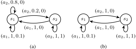
One obvious relaxed task for a given task is the deterministic version of the original task that preserves the set of nearoptimal policies. Figure 1 shows an example where the optimal policy of the deterministic relaxed task L′ is the optimal policy of the original L. Clearly, it is far easier to find out the optimal policy in L′ than in L. By Lemma 3.3, if RMAX explores in L with m = mL′ = 1 as if it is in L′ , it may converge to the optimal policy of L with much fewer samples. However, if the self-transition (s1, a2, s1) happens before (s1, a2, s2) in L, then the resulting trajectory can never be yielded in the corresponding deterministic L′ , and it is less likely that R-MAX still keeps to be PAC-MDP thereafter. Therefore, the corresponding probability pL′ can be fairly small in this case.
Usually, the non-deterministic relaxed tasks can have much higher pL′ than the deterministic one. Nevertheless, because the probability 1-pL′ is still non-trivial, if any strategywants to exploit these relaxed tasks and be PAC-MDP simultaneously, it must have some mechanisms to correct undesirable exploration behavior caused by the difference between the original task and its relaxed tasks. This is the reason we introduce the re-optimisticalization operation to ICR.
Now we are ready for the new upper bound for ICR.
Theorem 3.4. Given an arbitrary learning task L = (S,A, T,R, γ, ε, δ) and its K + 1 relaxed tasks (L0, pL0 ,mL0 ), (L1, pL1 ,mL1 ), ..., (LK, pLK ,mLK ) where LK = L and pLK = 1. Without loss of generality, assume that mL0 < mL1 < ... < mLK . If the environment is able to accurately predict whether the executing ICR with current mt = mLi , seen as an R-MAX with m = mLi , is producing a trajectory in L which could be produced in Li as well, and send this information as a signal to ICR, so that ICR can stop increasing mt by setting mmax ← mt, then with probability at least 1δ, the expected sample complexity for ICR executed in L with initial parameter setting according to Theorem 3.1 is bounded by
Proof. (sketch) The whole learning process can be seen as a binary process with different success probability pL0 , pL1 , ..., pLK , where ICR tries successively to produce a trajectory that can be produced by R-MAX in L0, L1, ...,LK respectively with m = mL0 ,mL1 , ...,mLK . Therefore, the probability of ICR getting its first success at ⌊mt⌋ = mLi is given by P0 = pL0 for i = 0 and Pi = [∏i-1 j=0 (1 - pLj )]pLi for i > 0. After a success event at mt = mLi , ICR starts behaving exactly as R-MAX with m = mLi in L as if it is in Li. By Theorem 3.1 and Lemma 3.3, with probability at least 1 - δ, the sample complexity of this sub-trajectory is ˜O(CLi mLi ). With a linear increasing method, the additional overhead before mt reaches mLi is ˜O(CLmLi ), which is no larger than ˜O(CLi mLi ). Therefore, with probability at least (1 - δ)Pi , ICR has a sample complexity of ˜O(CLmLi ). Then Theorem 3.4 follows immediately.
At first glance, the assumption of additional signal seems unrealistic. However, in practical use, an algorithm is halted subject to some predefined conditions rather than runs for infinite steps. This halting signal is actually more informative than the one appeared in Theorem 3.4, as the halting signal contains information related to the performance of the current policy. Still, the sample complexity theories concern infinitestep situations, and consequently the halting signal needs to be revised into a non-stopping form, resulting in the weaker signal in Theorem 3.4.
Generally speaking, specifying all possible relaxed tasks for a given task is non-trivial, as there can be infinitely many relaxed tasks. Fortunately, there is no need for ICR to know them in prior, since a linear increasing mt eventually covers all possible integers between m0 and mL, and thus covers all relaxed tasks that is useful for ICR. Therefore, given an arbitrary task L, its relaxed tasks can be simply seen as a vector of probabilities (p1, p2, ..., pmmax ) where pk corresponds to pL′ that mL′ = k. Then the new bound can be written as ˜O( |S||A|Vmax ε(1-γ) (p1 + ∑mmax k=2 [∏k-1 j=1 (1 - pj)]pkk)). The probabilities (p1, p2, ..., pmmax ) can be obtained from empirical results as in Section 4.2. In many real-world domains, the non-deterministic property of the dynamics comes mostly from sensor noise or partial observability. Learning tasks in these domains can be easily relaxed to the easier ones where the agent could receive more accurate information, and thus it is very likely that most of the p1, p2, ..., pmmax are non-zero for these tasks. As the term [∏k-1 j=1 (1 - pj)]pkk decays almost exponentially with k, the main part of the bound above is almost linear to the relevant quantities of the learning task, showing that ICR is able to cut off overly cautious exploration efficiently most of the time.
3.3 Increasingly Cautious V-MAX (ICV)
The principle of ICO can also be applied to V-MAX, yielding the new exploration strategy of Increasingly Cautious VMAX (ICV). We replace the fixed m in the original biased transition in Equation 5 with the increasing ⌊mt⌋:
The resulting pseudo-code for ICV is given in Algorithm 2.
By combining the mechanism of V-MAX and ICO, ICV not only makes use of learned knowledge in early stages as V-MAX, but also reduces possible overly cautious sampling. PAC-MDP analysis for ICV can be done in the same way as ICR, showing that the bounds in Theorem 3.1 and Theorem 3.4 holds for ICV subject to the same conditions as ICR.
4 Experiments
In this section, we first introduce the basic settings of our experiments, then present the results in two parts. The first part demonstrates the overall performance improvement of ICR and ICV in complex problems; the second part illustrates how ICO utilizes the properties of a learning task in detail.
Algorithm 2 Increasingly Cautious V-MAX(m0, Δm, mmax)
- 1: Multiset of collected samples ψ ← ∅
˜
- 2: Initialize T , ˜R using Equation 7, 4
- 3: ˜Q(s, a) ← Vmax for all (s, a)
- 4: for timestep t = 1, 2, 3, ... do
- 5: Observe current state st
- 6: Execute greedy action at ← argmaxa ˜Q(st, a)
- 7: Receive reward rt and transit to the next state st+1
- 8: ψ ←ψ ∪ (st, at, st+1, rt)
- 9: mt ←min(mt-1 +Δm,mmax)
- 10: if ⌊mt⌋ > ⌊mt-1⌋ then
˜
- 11: Update T for all (s, a) that n(s, a) ≤ ⌊mt⌋ using Equation 7
- 12: if n(st, at) ≤ mmax then
˜
- 13: Update T (st, at, ·), ˜R(st, at, ·) using Equation 7, 4
˜
- 14: Update ˜Q by VI if T has been updated
In our experiments, the average number of timesteps the agent needs to discover a near-optimal policy, rather than the average cumulative reward, is used as performance metric, as the former is more suitable in the context of comparing the sampling efficiency of exploration strategies. Specifically, in each independent run of a learning process, the agent starts learning from a fixed start state, and a separate test process is carried out for every 100 learning steps to check if the agent has discovered a near-optimal policy. In the test process, the current policy πt is calculated by VI from a model built from all collected samples (even if the strategy has discarded them) without any optimism (so that exploration is turned off). Then, πt is assessed in 20 independent test runs, each for 1000 steps from the start state; the average per-step reward ρπt can be estimated from these test runs. If the result is no less than 0.9ρ∗ , where ρ∗ is the average per-step reward of the optimal policy, then we say that the agent yields a success in discovering a 0.1ρ∗ -optimal policy, and the current timestep τ is reported as the final result of this learning process. If the agent fails to find out a 0.1ρ∗ -optimal policy within tmax = 300000 steps, then a timeout is reported.
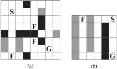
We conducted our experiments in a maze-style domain called ComplexMaze, which combines the key elements of FlagMaze [Dearden et al., 1998] and MazeWithPits [Leffler et al., 2007]. In a ComplexMaze, the task of the learning agent is to find out sufficient policies that collect all flags and reach goal in fewer steps without falling into any pits. Flags and pits are compact alternatives respectively for suboptimal goals [Wiering and Schmidhuber, 1998] and combination locks [Whitehead, 1991; Li, 2012], which make exploration more challenging. Some examples of the ComplexMaze we used are shown in Figure 2.
We used a continuing task setting with γ = 0.998. The agent starts from the grid marked as 'S' with no collected flags; in every time step, the agent must choose to move to one of the four possible directions. The probability p of slipping events, where an agent slips into one of the two wrong directions perpendicular to the chosen direction, was set to 0.1 as in FlagMaze. The reward for reaching the goal 'G', rgoal, is in the form of cnflags , where c is a constant and nflags is the number of collected flags. After receiving the goal reward, all collected flags will be reset and the agent will be sent back to 'S'. Pits (displayed as gray grids) work in the same way as the goal, except their rewards are always zero. Walking toward blocks (displayed as black grids) or borders of the maze has no effect on position, flags or reward. As long as γ < 1, longer paths are penalized by the discount, so a trivial step penalty is not necessary. The threshold of the Bellman error in Value Iteration was set to 0.01.
4.1 Experiments for overall performance
We compared the performance of ICR and ICV with R-MAX, V-MAX, as well as OIM [Szita and L˝orincz, 2008], which is reported to have good empirical results in various domains, and MoRMAX [Szita and Szepesv´ari, 2010], which has a better sample complexity upper bound than R-MAX. The maze shown in Figure 2 (a) was used with rgoal = 10nflags . Under this setting, a 0.1ρ∗ -optimal policy must collect all flags and avoid all pits before reaching the goal, and only about 4 suboptimal roundabout steps is allowed in the path connecting the start and the goal. Without a surprise, ε-greedy yielded timeouts in all 20 runs respectively under all tested parameters, indicating that the learning task is far from trivial.
By trial-and-error on the parameters, we found that setting m = 5 for R-MAX and V-MAX produces best results in this learning task. Setting m < 5, on the other hand, will notably increase the chances of timeouts. Rao and Whiteson [2012] suggest that unlike R-MAX, setting m large for V-MAX will not worsen its performance. However, with m = 1000, m = 10000 and m = tmax, V-MAX (as well as R-MAX) yielded timeouts in all 20 runs in both mazes shown in Figure 2 (a) and (b), indicating that V-MAX with large m performs as poorly as R-MAX against combination locks. The best parameter found for OIM is R0 = 0.05Rmax, and for MoRMAX is m = 3. For ICR and ICV, although there seem to be three parameters, we found that a trivial setting of m0 = 2, mmax = tmax is sufficient for all tasks in our experiments. Meanwhile, the best Δm found was 1/7000 for ICR and 1/5000 for ICV.
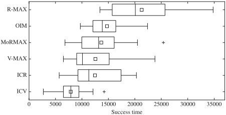
The results of success time τ in the 20 runs are shown in the box plot in Figure 3. On average, ICR and ICV had an improvement of 71.0% and 59.1% respectively to their original versions. The result of Friedman test is p = 3.9 × 10⁻¹⁰ , suggesting the difference between the strategies is significant;
Success time
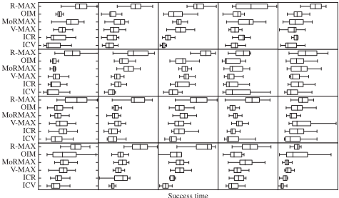
Figure 4: Success time τ in 20 generated mazes. Timeouts and outliers are not shown for the sake of clarity.
further multiple comparison by Tukey's range test shows that at significance level 0.1, ICV outperformed all other strategies, while ICR outperformed R-MAX and matched the performance of OIM, MoRMAX, and V-MAX.
We also conducted the same experiment on a set of 20 randomly generated 8×8 ComplexMazes. 1 Different patterns were observed: in some mazes, pits and flags are highly concentrated, requiring more cautious exploration, while in some others, pits and flags are clearly separated, and thus a careless exploration might be sufficient.
Considering that the scale of the problems are nearly identical, we used the same parameter settings as in the former experiment. As a result, R-MAX, V-MAX, and MoRMAX respectively yielded 5, 6, and 9 timeouts in 9 of the 20 mazes, while no timeout was reported for OIM, ICR or ICV. This indicates that compared with OIM, ICR and ICV, the optimal settings of parameter for R-MAX, V-MAX, and MoRMAX are more sensitive to the dynamics of the problems, and therefore careful parameter tuning is required for these strategies. The success time τ in 20 mazes are shown in the box plots in Figure 4.
Two-way rank transform ANOVA test with an additive model shows that the p-values for the strategies, the mazes, and the interaction between them are all less than 1.7×10⁻¹⁷ .
1 Details can be found at http://staff.ustc.edu.cn/~ketang/codes/ IJCAI15ICO.html
This suggests that all of these factors had significant impact on the results, and thus our 20-maze setting is meaningful for comparing overall performance of the strategies. Further multiple comparison shows that at significance level 0.05, ICV outperformed all other strategies, ICR outperformed all except ICV, while OIM, MoRMAX and V-MAX were in a tie, and R-MAX was dominated by all.
4.2 Illustrating the Utilization of Relaxed Tasks
In Section 3.2, we mentioned that given an arbitrary learning task, its relaxed task probability vector can be obtained from empirical results. In this experiment, we measure this probability vector for the maze domain shown in Figure 2 (b) to demonstrate how this can be done, and use the results to illustrate how ICO works in detail.
Under our experiment setting, the relaxed tasks can be seen as a relationship between τLi , mLi and pLi , such that (1) τLi is positively related to mLi , and (2) for R-MAX with m = mLi , with probability pLi , it finds out a 0.1ρ∗ -optimal policy with τLi steps in average; otherwise it converges to an undesirable policy and yields a timeout. Then the probability ICR discovers a 0.1ρ∗ -optimal policy at ⌊mt⌋ = mLi can be estimated from the observed ¯ pLi by ˆ P0 = ¯ pL0 and ˆ Pi = [∏i-1 j=0 (1 - ¯ pLj )] ¯ pLi for i > 0. The estimated value of ˆ Pi should be consistent with the observed ˜ Pi if the probability pLi we measure here is essentially the same thing in Definition 3.2.
The experiment was carried out in the ComplexMaze shown in Figure 2 (b) with rgoal = 1000nflags ; this task resembles the widely used Chain domain [Meuleau and Bourgine, 1999]. As our ICR does not discard samples collected for known-for-now state-action pairs, in order to reduce the variables of the experiment, we compared ICR with a nondiscarding version of R-MAX. The results of 40 independent runs for R-MAX respectively with m = 2, 3, 4, 5 and ICR with m0 = 2, Δm = 1/2400,mmax = tmax are shown in Table 1.
| mLi | 2 | 3 | 4 | 5 | |
|---|---|---|---|---|---|
| R-MAX | ¯ τLi ¯ | 2600.0 | 3676.5 | 4700.0 | 5905.0 |
| pLi ˆ | 19/40 | 34/40 | 39/40 | 40/40 | |
| Pi | 47.5% | 44.6% | 7.7% | 0.2% | |
| ICR | ˜ τLi ˜ | 2252.6 | 3841.2 | 6725.0 | 0.0 |
| Pi | 47.5% | 42.5% | 10.0% | 0.0% |
From the results of R-MAX, it can be observed that ¯ τi increases with mLi almost linearly, which is sensible because the possible route of exploration is highly constrained in this maze. The results of ¯ pLi suggests that the relaxed task probability vector of this maze domain is approximately (0, 0.475, 0.85, 0.975, 1). It can be inferred reasonably that the terms after p5 are also 1. The observed ˜ Pi of ICR is very close to their estimated value ˆ Pi made from ¯ pLi , supporting that the probability vector obtained above is a sufficient approximation to the true one defined in Section 3.2.
On the other hand, ˜ τi of ICR is not strictly consistent with ¯ τi of R-MAX due to the additional overheads in ICR and the non-overlapping intervals of ˜ τi. This suggests that the mechanisms of ICO is still improvable, as there is no mechanism for explicitly controlling the additional overheads yet.
The mean value of τ in all 40 runs for ICR is 3375.0 with no timeout occurred, outperforming R-MAX with any fixed m in probability (since timeouts indicate τ → +∞). These results support that by utilizing the relaxed task property of the learning problem, ICO is able to control the degree of cautiousness effectively and automatically.
5 Conclusion and Discussion
We have presented that by applying the principle of ICO to R-MAX and V-MAX, the newly proposed strategies ICR and ICV improve their original versions respectively both in theoretical guarantee and in empirical performance. Still, there is space for further improving ICR and ICV. The proof of the sample complexity bound for ICR in Theorem 3.1 actually does not concretely rely on certain style of increasing mt, and can be generalized to polynomial, logarithmic, or more complicated style of increasing with slight modification. This may help reducing the additional overheads caused by the linear style currently used in ICR and ICV.
The ICO is a general principle and could be applied to other PAC-MDP strategies, such as OIM, MBIE, MoRMAX, or even non-PAC-MDP strategies such as Bayesian Exploration Bonus [Kolter and Ng, 2009] which utilizes optimism under the Bayesian framework. We are particularly interested in applying ICO to MoRMAX, which may produce a strategy with the tightest sample complexity bound among the PAC-MDP strategies ever been published.
Finally, a combination of ICO and Knows What It Knows framework [Li et al., 2011] may lead to discovery of new strategies that are strong both in theory and in practice in continuous-space problems, as ICR and ICV in the discrete ones.
Acknowledgments
This work was supported in part by the 973 Program of China under Grant 2011CB707006, the National Natural Science Foundation of China under Grants 61175065 and 61329302, the Program for New Century Excellent Talents in University under Grant NCET-12-0512, the European Union Seventh Framework Programme under Grant 247619, and an EPSRC grant (No. EP/I010297/1). Xin Yao was support by a Royal Society Wolfson Research Merit Award.
@inproceedings{ijcai2015p566,
  title     = {Increasingly Cautious Optimism for Practical PAC-MDP Exploration},
  author    = {Zhang, Liangpeng and Tang, Ke and Yao, Xin},
  booktitle = {Proceedings of the Twenty-Fourth International Joint Conference on
               Artificial Intelligence, {IJCAI-15}},
  publisher = {International Joint Conferences on Artificial Intelligence},
  editor    = {Qiang Yang and Michael Wooldridge},
  pages     = {4041--4047},
  year      = {2015},
  month     = {7},
  note      = {Special Track on Machine Learning},
  url       = {https://ijcai.org/proceedings/2015/566},
}
TY - CPAPER TI - Increasingly Cautious Optimism for Practical PAC-MDP Exploration AU - Zhang, Liangpeng AU - Tang, Ke AU - Yao, Xin T2 - Proceedings of the Twenty-Fourth International Joint Conference on Artificial Intelligence, IJCAI-15 PB - International Joint Conferences on Artificial Intelligence PY - 2015 SP - 4041 EP - 4047 UR - https://ijcai.org/proceedings/2015/566 ER -Copied
Machine-readable versions of this paper, for tools and AI agents:





