
A Direct Boosting Approach for Semi-supervised Classification
Proceedings of the Twenty-Fourth International Joint Conference on Artificial Intelligence. Special Track on Machine Learning. Pages 4033-4039.
© 2015 International Joint Conferences on Artificial Intelligence
Abstract
We introduce a semi-supervised boosting approach (SSDBoost), which directly minimizes the classification errors and maximizes the margins on both labeled and unlabeled samples, without resorting to any upper bounds or approximations. A two-step algorithm based on coordinate descent/ascent is proposed to implement SSDBoost. Experiments on a number of UCI datasets and synthetic data show that SSDBoost gives competitive or superior results over the state-of-the-art supervised and semi-supervised boosting algorithms in the cases that the labeled data is limited, and it is very robust in noisy cases.
- [Appel et al., 2013] R. Appel, T. Fuchs, T. Dollar and P. Per- ona. Quickly boosting decision trees -Pruning under- achieving features early. International Conference on Machine Learning (ICML), 594-602, 2013.
- [Bennett et al., 2002] K. Bennett, A. Demiriz and R. Maclin. Exploiting unlabeled data in ensemble methods. Inter- national Conference on Knowledge Discovery and Data Mining (KDD), 289-296, 2002.
- [Bertsekas, 1998] D. Bertsekas. Network Optimization: Continuous and Discrete Models. Athena Scientific, 1998.
- [Chapelle et al., 2006] O. Chapelle, V. Sindhwani and S. Keerthi. Branch and bound for semi-supervised support vector machines. Advances in Neural Information Pro- cessing Systems (NIPS), 2006.
- [Chen and Wang, 2007] K. Chen and S. Wang. Regularized boost for semi-supervised learning. Advances in Neural Information Processing Systems (NIPS), 512-518, 2007.
- [Chen and Wang, 2011] K. Chen and S. Wang. Semi- supervised learning via regularized boosting working on multiple semi-supervised assumptions. Pattern Analysis and Machine Intelligence, IEEE Transactions on 33.1: 129-143, 2011.
- ['Alché-Buc et al., 2002] F. d'Alché-Buc, Y. Grandvalet and C. Ambroise. Semi-supervised marginBoost. Ad- vances in Neural Information Processing Systems (NIPS) 14, 553-560, 2002.
- [Demiriz et al., 2002] A. Demiriz, K. Bennett and J. Shawe- Taylor. Linear programming boosting via column gener- ation, Machine Learning, 46:225-254, 2002.
- [Frank and Asuncion, 2010] A. Frank and A. Asun- cion. UCI Machine Learning Repository. [http://archive.ics.uci.edu/ml], Irvine, CA: Univer- sity of California, School of Information and Computer Science, 2010. Link
- [Freund and Schapire, 1997] Y. Freund and R. Schapire. A decision-theoretic generalization of on-line learning and an application to boosting. Journal of Computer and Sys- tem Sciences, 55(1):119-139, 1997.
- [Joachims, 1999] T. Joachims. Transductive inference for text classification using support vector machines. Inter- national Conference on Machine Learning (ICML), 200- 209, 1999.
- [Long and Servedio, 2010] P. Long and R. Servedio. Ran- dom classification noise defeats all convex potential boosters. Machine Learning, 78:287-304, 2010.
- [Mallapragada et al., 2009] P. Mallapragada, R. Jin, A. Jain and Y. Liu. Semiboost: Boosting for semi-supervised learning. IEEE Trans. on Pattern Analysis and Machine Intelligence, 31(11):2000-2014, 2009.
- [Mason et al., 2000] L. Mason, J. Baxter, P. Bartlett and M. Frean. Boosting algorithms as gradient descent. Advances in Neural Information Processing Systems (NIPS), 512-518, 2000.
- [Mease and Wyner, 2008] D. Mease and A. Wyner. Evidence contrary to the statistical view of boosting. Journal of Machine Learning Research, 9:131-156, 2008.
- [Nguyen and Sanner, 2013] T. Nguyen and S. Sanner. Algo- rithms for direct 0-1 loss optimization in binary classifi- cation. International Conference on Machine Learning (ICML), 1085-1093, 2013.
- [Ratsch et al., 2000] G. Ratsch, T. Onoda and R. Muller. Soft margins for AdaBoost. Machine Learning, 1-35, 2000.
- [Rudin et al., 2004] C. Rudin, I. Daubechies and R. Schapire. The dynamics of AdaBoost: Cyclic behavior and convergence of margins. Journal of Machine Learning Research, 5:1557-1595, 2004.
- [Saffari et al., 2008] A. Saffari, H. Grabner and H. Bischof. SERBoost: Semi-supervised boosting with expectation regularization. European Conference on Computer Vision (ECCV), 588-601, 2008.
- [Schapire et al., 1998] R. Schapire, Y. Freund, P. Bartlett and W. Lee. Boosting the margin: A new explanation for the effectiveness of voting methods. The Annals of Statistics, 26(5):1651-1686, 1998.
- [Schapire and Freund, 2012] R. Schapire & Y. Freund. Boosting: Foundations and Algorithms. MIT Press, 2012.
- [Sindhwani et al., 2006] V. Sindhwani, S. Keerthi and O. Chapelle. Deterministic annealing for semi-supervised kernel machines. International Conference on Machine Learning (ICML), 841-848, 2006.
- [Tseng, 2001] P. Tseng. Convergence of block coordinate descent method for nondifferentiable minimization. Jour- nal of Optimization Theory and Applications, 475-494, 2001.
- [Vapnik, 1998] V. Vapnik. Statistical Learning Theory. John Wiley, 1998.
- [Warmuth et al., 2007] M. Warmuth, K. Glocer and G. Ratsch. Boosting algorithms for maximizing the soft margin. Advances in Neural Information Processing Sys- tems (NIPS), 1585-1592, 2007.
- [Zhai et al., 2013] S. Zhai, T. Xia, M. Tan and S. Wang. Di- rect 0-1 loss minimization and margin maximization with boosting. Advances in Neural Information Processing Systems (NIPS), 872-880, 2013.
- [Zheng et al., 2009] L. Zheng, S. Wang, Y. Liu and C. Lee. Information theoretic regularization for semi-supervised boosting. International Conference on Knowledge Dis- covery and Data Mining (KDD), 1017-1026, 2009.
References were extracted automatically from the PDF and may contain errors.
Full text extracted automatically from the PDF; figures, tables and equations may differ. The PDF is the version of record.
1 Introduction
In many applications of classifiers, labeled data is usually limited while unlabeled data can often be much cheaper and more plentiful than labeled data. Semi-supervised learning is a way to employ a large amount of unlabeled data together with a few labeled data to construct a classifier with good generalization.
Boosting, as an ensemble learning framework, is one of the most powerful classification algorithms in supervised learning. Based on the gradient descent view of boosting [Mason et al., 2000], many semi-supervised boosting methods have been proposed, such as SMarginBoost [d'Alch´e-Buc et al., 2002], ASSEMBLE [Bennett et al., 2002], RegBoost [Chen and Wang, 2007; Chen and Wang, 2011], SemiBoost [Mallapragada et al., 2009], SERBoost [Saffari et al., 2008] and information theoretic regularization based boosting [Zheng et al., 2009], where a margin loss function is minimized over both labeled and unlabeled data by the functional gradient descent method. The effectiveness of these methods can be ascribed to their tendency to produce large margin classifiers with a small classification error. However, these algorithms were not designed to directly maximize the margin (although some of them have the effects of margin enforcing), and the objective functions are not related to the margin in the sense that one can minimize these loss functions while simultaneously achieving a bad margin [Rudin et al., 2004]. Therefore, a natural goal is to construct classifiers that directly optimize margins as measured on both labeled and unlabeled data.
In this paper, we propose a new semi-supervised direct boosting method named SSDBoost that extends the work of DirectBoost [Zhai et al., 2013] to semi-supervised classification. The process of SSDBoost includes two steps: it first directly minimizes a generalized classification error that extends the concept of classification error to both labeled and unlabeled data, by iteratively adding base classifiers to the ensemble classifier. Once the generalized classification error reaches a coordinatewise local minimum 1 , it continuously adds base classifiers by directly maximizing a generalized average margin that consists of both labeled and unlabeled margins. The first step serves as an initialization method of the second step, the motivation is that the margin maximization algorithm often performs better when it starts with a low classification error.
Both SSDBoost and DirectBoost [Zhai et al., 2013] are coordinate optimizations in the hypothesis space, where only one coordinate is chosen and the corresponding parameter is updated at each iteration. However, SSDBoost is a nontrivial extension of DirectBoost to semi-supervised classification, where we have to mathematically re-formulated the semi-supervised boosting approach by extending the classification error and margin function to unlabeled data. Since the objectives in SSDBoost are more complicated, we designed new optimization techniques and provide the rationales behind our approach. We will show that SSDBoost is able to exploit easily-obtained unlabeled data to significantly improve accuracy, especially in the noisy cases. Due to space limitation, the proofs of properties and theorem are given in the supplementary material.
2 SSDBoost Algorithm
Let H = {h1, ..., h|H|} denote the set of all possible weak classifiers that can be produced by the weak learning algorithm, where a weak classifier hj ∈ H is a mapping from an instance space X to Y = {-1, 1}, and H is closed under negation, i.e., both h and -h belong to H. In this study, we use decision trees as the weak learning algorithm 2 , then |H| is finite but can be extremely large.
1 See the definition on page 479 in [Tseng, 2001].
2 As the combination of boosting with decision trees is the stateof-the-art approach [Appel et al., 2013].
Assume we are provided n labeled samples, Dl = {(x1, y1), · · · , (xn, yn)} and m unlabeled samples, Du = {xn+1, · · · , xN} (let N = n+m). Semi-supervised boosting combines weak classifiers to form a highly accurate ensemble classifier by using the combined training set D = Dl ∪ Du . Formally, for binary classification, the ensemble classifier is defined to be sign(f(x)), where f(x) = ∑h∈H αhh(x), αh ≥ 0 is the ensemble function. Our goal is to find an ensemble classifier that has good generalization performance. To this end, we developed a semi-supervised boosting approach through two steps. In the following, we will elaborate the two steps respectively.
2.1 Minimize generalized classification error
For the labeled data, the classification error (or 0-1 loss) is defined to be
where 1(·) is an indicator function. While optimizing the classification error is NP-hard, it is robust to noise [Nguyen and Sanner, 2013] and is consistent under certain conditions [Vapnik, 1998]. For Du , since the labels are unknown, a natural extension of the 0-1 loss is the expected classification error
Minimizing (2) has the effects to push p(y|x) away from 0.5, so that the uncertainty of the putative labels is reduced. For binary classification tasks, the logistic (sigmoid) function of yf(x), sigmoid(yf(xi)) = 1/(1+exp(-yf(xi))), is a good estimation of p(y|xi) [Schapire and Freund, 2012], and then the loss of the minimum entropy semi-supervised boosting method [Zheng et al., 2009] is a surrogate upper bound of (2). Combining (1) and (2), we have the generalized classification error
where γ is a trade-off parameter that controls the influence of the unlabeled data.
Consider the tth iteration, the ensemble function is
where previous t - 1 weak classifiers hk(x) and corresponding weights αk, k = 1, · · · , t - 1 have been selected and determined. Then for a given weak classifier ht(x), the goal is to choose its weight αt such that (3) is minimized. If we estimate p(y|xi) by sigmoid(yf(xi)), the second term of (3) is a complex function of αt, and thus it is difficult to compute the optimal αt. Instead, we estimate p(y|xi) by the logistic function of f of the previous step, sigmoid(yft-1(xi)), and update the estimation through an iterative scheme. We define ˆ error(f,Du ) to be 1m ∑Ni=n+1 ∑y∈Y ˆ p(y|xi)1(yf(xi) ≤ 0)
Algorithm 1 Minimize the generalized 0-1 loss on D.
- 1: Initialize: t = 0, ft(xi) = 0, i = 1, · · · ,N.
- 2: repeat
- 3: t ← t + 1.
- 4: ˆ p(y|xi) = sigmoid(yft-1(xi)) for xi ∈ Du .
- 5: Sort |ft-1(xi)|, xi ∈ D in an increasing order.
- 6: Pick a weak classifier ht by Algorithm 1-2.
- 7: Get the interval that has the minimum value of (5) by calling Algorithm 1-1 with ht, and set αt to be the value within this interval.
- 8: Update: ft(xi) = ft-1(xi) +αtht(xi).
- 9: until (5) reaches a local coordinatewise minimum.
- 10: Output: ft(xi).
Algorithm 1-1 Line search algorithm to find the interval with the minimum generalized 0-1 loss.
- 1: Input: a weak classifier ht ∈ H.
- 2: for i = 1, · · · ,N do
- 3: Compute the value of (5) at αt = 0.
- 4: Let ei = |ft-1(xi)|.
- 5: if (slope > 0 and intercept < 0), then error update on the righthand side of ei is - 1n for xi ∈ Dl or -γ |ˆ p(+1|xi)-ˆ p(-1|xi)| for xi ∈ Du .
- m 6: if (slope < 0 and intercept > 0), then error update on the righthand side of ei is 1n for xi ∈ Dl or γ |ˆ p(+1|xi)-ˆ p(-1|xi)| m for xi ∈ Du .
- 7: end for
- 8: Incrementally calculate (5) on intervals of ei's.
- 9: Output: the interval withminimumgeneralized 0-1 loss.
by replacing p(y|xi) in error(f,Du ) by ˆ p(y|xi). Therefore, the estimation of (3) is to be
which is a stepwise function of αt.
Algorithm 1 outlines a greedy coordinate descent algorithm to directly minimize (5). The line search algorithm, Algorithm 1-1, describes the way to find the optimal α for any given hypothesis h ∈ H such that (5) is minimized. The key is how to efficiently find the points that lead (5) changes. Denoting the inference function of a sample xi to be
which is a linear function with slope yht(xi) and intercept yft-1(xi). For a labeled sample (xi, yi), Ft(xi, yi) > 0 indicates this sample is correctly classified; otherwise, it is
misclassified. These two states exchange at the point αt = - ft-1(xi) ht(xi) , we denote this point as a critical point ei. Thus, the value of the generalized 0-1 loss (5) has 1n differences at ei. To compute the "classification error" of an unlabeled sample, we use ˆ yi = sign(ft-1(xi)) to denote its pseudo label. Similarly, the sign of Ft(xi, ˆ yi) identifies xi ∈ Du is "correctly classified" or "misclassified". Again, the critical point for xi ∈ Du is ei = - ft-1(xi) ht(xi) , and the value of (5) has
Algorithm 1-2 Weak learning algorithm.
- 1: Input: a training set D, current tree depth ℓ.
- 2: if ℓ ≤ max depth then
- 3: for a binary split do
- 4: Split D into Dleft and Dright, then a weak hypothesis h ∈ H is generated which maps Dleft to +1 and Dright to -1.
- 5: Call Algorithm 1-1 with h and its negation -h ∈ H respectively.
- 6: end for
- 7: Choose the optimal binary split which partitionsD into Dleft and Dright, update ht with the corresponding labels on Dleft and Dright.
- 8: Call weak learning algorithmwith Dleft and ℓ +1.
- 9: Call weak learning algorithmwith Dright and ℓ +1.
- 10: end if
- 11: Output: a weak classifier ht ∈ H.
γ |ˆ p(+1|xi)-ˆ p(-1|xi)| m differences at ei. Since H is closed under negation, we only care about the case that ei is greater than 0 (where ei = - ft-1(xi) ht(xi) = |ft-1(xi)|), that corresponds to the two scenarios described at line 5 and 6. The critical points divide αt into at most N + 1 intervals, each interval has the value of a generalized 0-1 loss (5). Since we visit each sample in an increasing order, the critical points are also in an increasing order.
Algorithm 1-2 describes the weak learning algorithm, where the decision trees with binary splits are used. We simply choose the attribute to split by minimizing (5), the whole process to build trees is a top-down, greedy search approach. Since ft-1 is used when building trees, Algorithm 1-2 will not end up with the same tree though SSDBoost does not maintain a distribution over training samples.
The complexity of Algorithm 1 is O(LN + N logN) for each iteration when decision stumps are used as weak learners 3 , where L is the number of binary splits. It has the same computational costs as the methods [Bennett et al., 2002; Zheng et al., 2009] which optimize surrogate losses. Algorithm 1 terminates at a coordinatewise local minimum of (5), SSDBoost then switches to the margin maximization step.
2.2 Maximize the generalized average margin
The success of boosting can be ascribed to margin maximization [Schapire et al., 1998], but most previous boosting approaches were not designed to explicitly optimize the margins [Schapire and Freund, 2012]. While some exceptions, such as LPBoost [Demiriz et al., 2002], SoftBoost [Warmuth et al., 2007], and DirectBoost [Zhai et al., 2013], specially maximize a relaxed hard margin objective, they are only designed for supervised classification. For the existing semi-supervised boosting methods [Bennett et al., 2002; Chen and Wang, 2007; d'Alch´e-Buc et al., 2002; Mallapragada et al., 2009; Saffari et al., 2008; Zheng et al., 2009], none of them has been shown to maximize the margins on Dl ∪ Du , although some of them employ margin enforcing loss functions. In this section, we introduce a generalized average margin on Dl ∪ Du , and propose a coordinate ascent algorithm that directly maximizes this objective function.
3 Decision stumps are the decision trees with a depth of 1. The computational costs of Algorithm 1 has the same increasing rate as the methods in [Bennett et al., 2002; Zheng et al., 2009] if large trees are considered.
The (normalized) margin of a labeled sample (xi, yi) w.r.t
preted as a measure of how confidently this labeled sample is correctly classified. For an unlabeled sample xi, it is natural to define its margin as the expected margin:
By sorting ϕli and ϕui in an increasing order respectively, and consider n′ worst labeled samples n′ ≤ n and m′ worst unlabeled samples m′ ≤ m that have smaller margins, then the generalized average margin over those samples is
where Bln′ denotes the set of n′ labeled samples having the smallest margins, and Bum′ denotes the set of m′ unlabeled samples having the smallest margins. The parameter n′ indicates how much we relax the hard margin on labeled samples, and we often set n′ based on knowledge of the number of noisy samples in Dl [Ratsch et al., 2000]. The higher the noise rate, the larger the n′ should be used. The parameter m′ controls the relaxation of the margin distribution over the unlabeled data. A smaller m′ makes the algorithm focus more on the unlabeled samples close to the decision boundary.
For an unlabeled sample xi, again we estimate p(y|xi) by ˆ p(y|xi) = sigmoid(yft-1(xi)). Denote ˆ yi = 2 1+e-(ft-1(xi)) -1, then the estimated margin of xi is
Thus, the objective function that we are working on in the margin maximization step is
The outline of the greedy coordinate ascent algorithm that sequentially maximizes (10) is described in Algorithm 2. We first sort ϕli=1,···,n and ˆ ϕui=n+1,···,N (line 5) in order to efficiently compute the optimal solution of maximum (10) we will explain later. At the iteration t, we select a weak classifier ht (line 6) and its weight αt (line 7) such that (10) is maximized. We repeat this process until (10) reaches a local coordinate maximum.
The key part in Algorithm 2 is the line search algorithm which finds the value of αt that maximizes (10) for a given weak classifier ht ∈ H. On the t-th iteration, let c = ∑t-1 k=1 αk, then the derivative of ϕli with respect to αt is calculated as,
Algorithm 2 Maximize margins on Dl ∪ Du .
- 1: Initialize: t and ft fromAlgorithm 1.
- 2: repeat
- 3: t ← t + 1.
- 4: Update ˆ yi = 2 1+e-ft-1(xi) -1, i = n+1, · · · ,N.
- 5: Sort ϕli=1,···,n and ˆ ϕui=n+1,···,N in increasing order at αt = 0 respectively, determine Bln′ and Bum′ .
- 6: Pick a weak classifier ht by weak learning algorithm.
- 7: Compute q∗ by Algorithm 2-1 that maximizes (10) along the coordinate ht. Set αt = q∗ .
- 8: Update ft(xi) = ft-1(xi) +αtht(xi).
- 9: until ˆ ϕavg(n′ ,m′ ) reaches a local coordinatewise maximum.
- 10: Output: ft(xi).
Since c ≥ yift-1(xi), depending on the sign of yiht(xi), (11) is either positive or negative, which is irrelevant to the value of αt. That is, if the labeled sample (xi, yi) ∈ Dl is correctly classified by ht (yiht > 0), then ϕli is monotonically increasing with respect to αt. Otherwise, ϕli is monotonically decreasing. Similarly, for an unlabeled sample xi, the derivative of ˆ ϕui is either positive or negative depending on the sign of ˆ yiht(xi), and which is irrelevant to the value of αt. Hence for an interval of αt with the fixed Bln′ and Bum′ , the derivative of (10) is
which sign is irrelevant to the value of αt. Thus, with the fixed Bln′ and Bum′ , ˆ ϕavg(n′ ,m′ ) is a monotonic function of αt, depending on the sign of the derivative in (12), it is maximized either on the left side or on the right side of the interval.
Along the ht coordinate, Bln′ and Bum′ are not always fixed, hence we need to check the values of αt that lead Bln′ or Bum′ to change. To address this, we first examine when the margins ϕli and ϕlj of two labeled samples (xi, yi) and (xj, yj) intersect. Since H is closed under negation, it is not necessary to consider the cases that their intersection is negative. Obviously ϕli and ϕlj never intersect when they are both increasing or decreasing 4 . Otherwise, ϕli and ϕlj intersect with
As ϕli 's are sorted in advance (Algorithm 2, line 5), we can compute the intersections that result in the change of Bln′ very efficiently by Property 1.
Property 1 All the points that lead Bln′ to change can be determined by computing the intersections of the jth highest increasing margin in Bln′ and jth smallest decreasing margin in the complementary set of Bln′ .
4 If ϕli and ϕlj are both increasing or decreasing, then the denominator of (13) is 0, that indicates the intersection will never happen.
Proof : Let (ϕlj )inc denotes the jth highest increasing margin in Bln′ at αt = 0, and (ϕlj )dec denotes the jth smallest decreasing margin in (Bln′ )c at αt = 0. Denoting qj to be the intersection of (ϕlj )inc and (ϕlj )dec.
For j = 1, it is obviously that (ϕlj )dec is the first margin in (Bln′)c that intersects with (ϕl1 )inc. Therefore, q1 leads Bln′ to change as (ϕlj )dec belongs to Bln′ and (ϕl1 )inc belongs to (Bln′)c on the rightside of q1.
Suppose the conclusion holds for j = k - 1. For j = k, since (ϕl1 )dec, · · · , (ϕlk-1 )dec belong to Bln′ already, the intersections of (ϕlk )inc and those margins do not lead Bln′ to change. Hence (ϕlk )dec is the first margin in (Bln′)c that intersects with (ϕlk )inc, and the intersection qk leads Bln′ to change.
In addition, the following properties indicate that we do not need to consider the cases that the margins of two unlabeled data are both increasing or decreasing.
Property 2 If ˆ ϕui and ˆ ϕuj are both increasing, then they never intersect when αt > 0.
Proof : For any unlabeled sample x ∈ Du , ˆ y = 2 1+e-ft-1(x) -1 is a strictly monotonic function with ft-1(x), and ft-1(x)ˆ y ≥ 0 always holds.
Without loss of generality, we assume ft-1(xi) > ft-1(xj), then ˆ yjft-1(xj) - ˆ yift-1(xi) < 0. Since ϕui and ϕuj are both increasing, we have ht(xi)ft-1(xi) > 0, ht(xj)ft-1(xj) > 0, and ht(xi)ˆ yi > ht(xj)ˆ yj > 0. Thus,
That indicates ϕui intersects ϕuj at αt < 0.
Property 3 If ˆ ϕui and ˆ ϕuj are both decreasing, then they only intersect each other after intersecting with all the increasing margins.
Proof : For any decreasingmargins ϕui andϕuj in (Bum′)c , and any increasingmargin ϕuk in Bum′ . If we assume ϕui intersects ϕuk at qi,k, ϕuj intersects ϕuk at qj,k, and ϕui intersects ϕuj at qi,j, it is suffices to show qi,j > qi,k and qi,j > qj,k.
Since ϕui > ϕuk and ϕuj > ϕuk , then ft-1(xj) > ft-1(xk). Thus we have
We can prove the case qj,k < qi,j in the same way.
Thus, the points that lead Bum′ to change can be computed in the similar way as described in Property 1.
Based on the above discussion, we are able to efficiently compute all the intersections that lead Bln′ or Bum′ to change
(denoting these points as qj's), and we know that one of them is the optimal value of αt that maximizes (10) along the ht coordinate (denoting the optimal point as q∗ ). The next challenge is how to efficiently find q∗ among those qj 's. The computational cost of the straightforward solution in worst case is O((n′ +m′ )2 ) since there are at most n′ +m′ intersections and we have to compute (10) for each of them. Fortunately, we can prove that (10) is a quasi-concave function for any given weak hypothesis (in Theorem 1), that allows us to determine q∗ by incrementally updating (12) and checking its sign in O(n′ + m′ ). Specifically, if ∂ ˆ ϕavg(n′ ,m′ ) ∂qj > 0 and ∂ ˆ ϕavg(n′ ,m′ ) ∂qj+1 < 0, then q∗ = qj.
Theorem 1 Denote the average margin of the bottom n′ labeled samples and m′ unlabeled samples as
where {Bln′ |αt} denotes the set of n′ labeled samples whose margins are smallest for a fixed αt, and {Bum′ |αt} denotes the set of m′ unlabeled samples whose margins are smallest for a fixed αt. Then ˆ ϕavg(n′ ,m′ )(αt) is quasiconcave.
Proof (outline) : Let S = {αt : αt > 0}, which is a convex set. By definition of quasiconcave, ˆ ϕavg(n′ ,m′ ) is quasiconcave on S if and only if its upper contour sets are convex sets on S. The µ-upper-contour set Sµ of ˆ ϕavg(n′ ,m′ ) on S is denoted as
We now prove that Sµ is a convex set. For ∀α(1) t , α(2) t ∈ Sµ and ∀λ ∈ [0, 1], letting θ = (1-λ)α(1) t +λα(2) t then we have
Therefore, θ ∈ Sµ. ˆ ϕavg(n′ ,m′ )(αt) is quasiconcave.
Formally, the line search algorithm to calculate the value of q∗ is described in Algorithm 2-1. The way to select the weak classifier is very similar to Algorithm 1-2, the only modification is to replace the line search algorithm to Algorithm 2-1. Since ˆ ϕavg(n′ ,m′ ) is bounded, apparently Algorithm 2 converges to a coordinatewise local maximum. If there are L possible binary splits, the computational cost of Algorithm 2 is O(L(n′ + m′ ) + N log N) on each round.
Since ˆ ϕavg(n′ ,m′ ) is non-differentiable at the intersections, the coordinate ascent algorithm may get stuck at a corner from which it is impossible to make progress along any coordinate direction. To overcome this difficulty, we employ an ϵ-relaxation method [Bertsekas, 1998]. The main idea is to allow a single coordinate to change even if this worsens the objective function. When a coordinate is changed, however, Algorithm 2-1 Compute the q∗ that corresponds to the maximum of ˆ ϕavg(n′ ,m′ ).
- 1: Input: a weak classifier ht ∈ H.
- 2: Compute the value of (12) at αt = 0.
- 3: j ← 0, k ← 0, qj+k ← 0.
- 4: Compute the intersection qlj+1 of the j + 1th highest increasing margin in Bln′ and the j + 1th smallest decreasing margin in (Bln′ )c .
- 5: Compute the intersection qu k+1 of the k + 1th highest increasing margin in Bum′ and the k+1th smallest decreasing margin in (Bum′ )c .
- 6: qj+k+1 ←min(qlj+1 , qu k+1 ).
- 7: if ∂ ˆ ϕavg(n′ ,m′ ) ∂qj+k+1 > 0 then
- 8: if qlj+1 < qu k+1 then Incrementally update Bln′ and (12) at αt = qj+k+1; j ← j + 1.
- 9: else Incrementally update Bum′ and (12) at αt = qj+k+1; k ← k + 1.
- 10: Go back to line 4.
- 11: else
- 12: q∗ = qj+k, compute ˆ ϕavg(n′ ,m′ ) at q∗ .
- 13: end if
- 14: Output: q∗ .
it is set to ϵ plus the value that maximizes the margin function along that coordinate, where ϵ is a positive number. If ϵ is small enough, the algorithm can eventually approach a small neighborhood of the optimal solution.
3 Experiments
In this section, we first evaluate the performance of SSDBoost on 10 UCI datasets from the UCI repository [Frank and Asuncion, 2010], then examine its noise robustness on two datasets with random label noise. For comparison, we also report the results of several existing supervised boosting methods (AdaBoost [Freund and Schapire, 1997], LPBoost [Demiriz et al., 2002], and DirectBoost [Zhai et al., 2013]) and semi-supervised boosting methods (ASSEMBLE [Bennett et al., 2002] and semi-supervised entropy regularized boosting [Zheng et al., 2009] (denoted as SERBoost)). For all the algorithms in the comparison, we use decision trees as the weak learners. Note that it is not our intention to show that the proposed algorithm always outperforms a variety of supervised and semi-supervised learning methods. Instead, the empirical study is focused on whether the proposed SSDBoost is able to effectively improve the accuracy of the wellknown boosting algorithms with the same weak hypothesis space H. Thus, same as the ways the authors did in [Bennett et al., 2002; Chen and Wang, 2007; Demiriz et al., 2002; Zheng et al., 2009], we restrict the comparison with only boosting methods and the same weak learning algorithm, rather than other related works, such as Semi-Supervised Support Vector Machines (S3VM) [Chapelle et al., 2006; Joachims, 1999; Sindhwani et al., 2006].
| Data | M | D | AdaBoost | LPBoost | DirectBoost | ASSEMBLE | EntropyBoost | SSDBoost |
|---|---|---|---|---|---|---|---|---|
| Adult | 48842 | 14 | 15.11 (0.7) | 15.42 (1.0) | 15.08 (1.0) | 15.27 (0.9) | 14.97 (0.7) | 15.10 (0.8) |
| Australian | 690 | 14 | 17.83 (2.7) | 17.83 (2.5) | 16.38 (2.5) | 16.96 (2.2) | 17.07 (2.6) | 15.8 (2.6) |
| Kr-vs-kp | 3196 | 36 | 3.98 (0.8) | 4.01 (1.2) | 3.89 (0.9) | 3.45 (1.1) | 3.39 (1.4) | 3.39 (0.5) |
| Liver | 345 | 7 | 36.76 (3.4) | 38.53 (4.9) | 36.65 (4.4) | 36.18 (3.7) | 36.35 (4.9) | 33.24 (7.3) |
| Mushroom | 8124 | 22 | 0.1 (0.1) | 0.9 (0.5) | 0.18 (0.2) | 0.11 (0.1) | 0.12 (0.1) | 0.16 (0.2) |
| Sonar | 208 | 60 | 33.33 (5.2) | 32.22 (6.6) | 31.11 (5.6) | 28.33 (3.6) | 28.89 (4.1) | 28.44 (5.2) |
| Spambase | 4601 | 57 | 7.5 (0.9) | 7.52 (0.8) | 7.35 (1.1) | 7.48 (0.7) | 7.87 (0.9) | 7.09 (1.4) |
| Splice | 3190 | 61 | 14.6 (2.7) | 15.3 (2.2) | 14.6 (2.8) | 14.8 (2.7) | 14.9 (2.7) | 12.0 (1.7) |
| WDBC | 569 | 31 | 6.55 (1.6) | 6.94 (1.9) | 6.94 (1.8) | 7.54 (2.1) | 7.73 (2.1) | 6.15 (1.8) |
| WPBC | 198 | 34 | 33.68 (4.8) | 34.21 (6.0) | 32.63 (3.7) | 28.95 (4.4) | 29.68 (5.7) | 28.95 (3.8) |
| Data | AdaBoost | LPBoost | DirectBoost | ASSEMBLE | EntropyBoost | SSDBoost |
|---|---|---|---|---|---|---|
| Kr-vs-kp (50) | 10.46 (2.2) | 9.9 (2.4) | 9.66 (2.4) | 8.2 (2.2) | 8.5 (2.1) | 7.65 (2.0) |
| Mushroom (20) | 8.81 (1.9) | 9.7 (1.8) | 7.38 (1.8) | 5.05 (0.7) | 5.1 (1.6) | 2.2 (0.5) |
The classification error is estimated by 10-fold crossvalidation. For each dataset, we partition it into 10 parts evenly. In each fold, we use eight parts for training, one part for validation 5 , and the remaining part for testing. Within the eight parts of training data, only one part is used as labeled data, and the other parts are treated as unlabeled data (by simply discarding the labels). Since we concentrate on the cases where the labeled data are limited while the unlabeled data are adequate in the training process, the datasets we selected include datasets of small or moderate sizes, and only a small part (one tenth) is used as labeled data.
5 We use the validation data to choose the optimal model for all the methods. For each boosting method, the depth of decision trees is chosen from 1, 2, and 3 by the validation set (for the datasets in the experiments, decision trees with a depth of 1-3 are sufficient to produce good results). For AdaBoost, ASSEMBLE, and SERBoost, the validation data is also used to perform early stopping since overfitting is observed for these methods. We run these algorithms with a maximum of 3000 iterations, and then choose the ensemble classifier from the round with minimal error on the validation data. For ASSEMBLE, SERBoost, and SSDBoost, the trade-off parameters that control the influence of unlabeled data are chosen from the values {0.001, 0.01, 0.1, 1} by the validation data. For LPBoost, DirectBoost, and SSDBoost, the parameter n′ is chosen by the validation set from the values {n/10, n/5, n/3, n/2}. For SSDBoost, the parameter m′ is chosen from the values {m/10,m/5,m/3,m/2}, and ϵ is fixed to be 0.01 since it does not significantly affect the performance as long as its value was a small number. It is hard to accurately estimate parameters over a small validation set, but we found experimentally that it still has certain instructive effects on the quality of the classifiers.
3.1 UCI datasets
Table 1 shows, as we expected, the semi-supervised boosting algorithms (ASSEMBLE, EntropyBoost, and SSDBoost) outperform the supervised methods (AdaBoost, LPBoost, and DirectBoost) in general, the results indicate that the unlabeled data does help to improve generalization performance. By taking advantage of maximizing margins directly on both labeled and unlabeled data, SSDBoost gives the most accurate results (highlighted in bold font) in 7 of the 10 datasets among all the methods, and its results are close to the best results produced by the other methods for the remaining 3 datasets. We have also performed a significance test using the paired t-test. When compared to AdaBoost, SSDBoost has statistically significant improvements (p-value is less than 0.05) on Australian, Splice, and WPBC datasets.
We noticed that for some moderate size of datasets (such as Adult, Mushroom, and Kr-vs-Kp), the semi-supervised boosting methods do not provide much improvements. We believe the reason that there was little improvement for those datasets is that the numbers of labeled samples are enough to get reasonable results, so there is little room in the classification to improve accuracy further. We selected two datasets, Kr-vs-kp and Mushrooms, and we tried to reduce their size in order to show the power of semi-supervised learning. Table 2 shows the results of Kr-vs-kp and Mushroom datasets with 50 and 20 labeled samples respectively. When the labeled data is extremely limited, semi-supervised methods show their advantage more clearly, and SSDBoost is very efficient at utilizing the information of unlabeled data.
| Data | η | AdaBoost | LPBoost | DirectBoost | ASSEMBLE | EntropyBoost | SSDBoost |
|---|---|---|---|---|---|---|---|
| Synthetic | 0 | 13.12(1.6) | 13.96(1.7) | 12.6(1.2) | 12.28(2.5) | 11.8(1.0) | 10.04(1.7) |
| 0.05 | 19.52(3.9) | 19.36(4.9) | 16.56(3.7) | 16.92(2.7) | 17.88(3.9) | 14(2.6) | |
| 0.2 | 29.08(3.1) | 22.84(5.4) | 22.12(4.6) | 25.68(3.1) | 25.52(5.5) | 18(2.4) | |
| Kr-vs-Kp | 0 | 10.42(2.2) | 9.96(3.1) | 10.08(4.1) | 8.2(2.8) | 8.36(2.6) | 7.72(2.2) |
| 0.05 | 18.26(5.1) | 18.0(9.4) | 17.1(7.9) | 16.66(5.8) | 17.14(7.0) | 13.42(6.3) | |
| 0.2 | 27.18(8.3) | 25.58(7.2) | 22.46(7.7) | 20.84(7.7) | 21.4(7.5) | 16.06(7.4) |
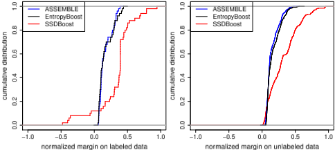
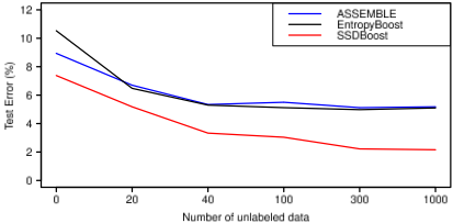
Figure 1 shows the test errors on the Mushroom dataset (with 20 labeled samples) using ASSEMBLE, EntropyBoost and SSDBoost when we increase the size of unlabeled data. This results indicate that the accuracy of semi-supervised boosting tends to improve with the increment of unlabeled data, but the effects become saturated when more unlabeled samples are added. We also observed this phenomenon on other datasets, and the same observation was made by the authors of [Zheng et al., 2009]. Moreover, SSDBoost consistently outperforms the other two in the cases that different numbers of unlabeled data are added to the training set.
We now analyze the running times of the semi-supervised boosting algorithms on Adult dataset, which has 4884 labeled and 34188 unlabeled training samples. We implemented each semi-supervised boosting algorithm by C++, and the decision trees with depth of 2 are used. ASSEMBLE and EntropyBoost take almost the same running time (about 1.4s) on each round in training phase. For SSDBoost 6 , it takes about 1.7s on each round, which is slightly slower than the other two but it is bearable on such a scale dataset. When compared to ASSEMBLE and EntropyBoost, SSDBoost has more parameters to tune. In practice, however, we used the following strategy to save the validation time: we adjusted n′ and m′ together from the 4 candidates {(n/10, m/10), (n/5, m/5), (n/3, m/3), (n/2, m/2)} instead of 16 combinations. In test phase, all the boosting methods have a similar computational time.
6 The running time includes both step 1 and step 2, which was computed by (total running time) / (total # of iterations).
3.2 Evaluation of Noise Robustness
In many real-world applications, robustness of a classifier is quite desirable. In this section, we run each boosting algorithm on the datasets with additional random label noise. We first use synthetic data with 5 real valued features which are generated by the model introduced in [Mease and Wyner, 2008]. In the experiments, we let the number of labeled, unlabeled training, validation and testing data be 50, 500, 50, 500 respectively, and the labels of the labeled training data are corrupted with a noise rate η at 0%, 5% and 20%. The experiments are repeated 10 times. In addition, we use Krvs-Kp dataset again, but this time we flip the labels of the labeled training data by a noise rate η. Table 3 shows the results of each boosting algorithm. Similar to AdaBoost, ASSEMBLE and EntropyBoost are very sensitive to noise [Long and Servedio, 2010], their accuracy is hurt even with a 5% noise rate. In contrast, the algorithms that maximize the average bottom samples (including LPBoost, DirectBoost, and SSDBoost) perform much better on the noisy cases. Particularly, SSDBoost does very well by utilizing the unlabeled data.
Figure 2 shows the cumulative margin distributions on Dl and Du respectively of semi-supervised boosting methods on the synthetic data with 20% label noise, where the margins of unlabeled data are measured in (8). For the margin distribution of labeled samples, as shown in the left panel, ASSEMBLE and EntropyBoost concentrate their resources on a few difficult samples, but these samples are usually noisy. SSDBoost allows some misclassifications to achieve a better margin distribution as well as generalization performance. For the margin distribution of unlabeled data, as shown in the right panel, we observed a similar interesting phenomenon. ASSEMBLE and EntropyBoost have slightly greater margins when considering the bottom 20% unlabeled samples, but SSDBoost achieves a better margin distribution overall.
4 Conclusion
We have proposed a semi-supervised boosting method that directly optimizes classification errors and margins on both available labeled and unlabeled data. Coordinate descent/ascent based optimization algorithms are proposed to facilitate this idea. The results on both UCI datasets and a synthetic noisy dataset demonstrate the feasibility and advantages of this approach, and the observed robustness of SSDBoost suggests that it might be quite useful in practice.
Acknowledgments
This research is supported in part by AFOSR under grant FA9550-10-1-0335, NSF under grant IIS:RI-small 1218863, DoD under grant FA2386-13-1-3023, and a Google research award. We would like to thank the Ohio Supercomputer Center for an allocation of computing time to make this research possible.
@inproceedings{ijcai2015p565,
  title     = {A Direct Boosting Approach for Semi-supervised Classification},
  author    = {Zhai, Shaodan and Xia, Tian and Li, Zhongliang and Wang, Shaojun},
  booktitle = {Proceedings of the Twenty-Fourth International Joint Conference on
               Artificial Intelligence, {IJCAI-15}},
  publisher = {International Joint Conferences on Artificial Intelligence},
  editor    = {Qiang Yang and Michael Wooldridge},
  pages     = {4033--4039},
  year      = {2015},
  month     = {7},
  note      = {Special Track on Machine Learning},
  url       = {https://ijcai.org/proceedings/2015/565},
}
TY - CPAPER TI - A Direct Boosting Approach for Semi-supervised Classification AU - Zhai, Shaodan AU - Xia, Tian AU - Li, Zhongliang AU - Wang, Shaojun T2 - Proceedings of the Twenty-Fourth International Joint Conference on Artificial Intelligence, IJCAI-15 PB - International Joint Conferences on Artificial Intelligence PY - 2015 SP - 4033 EP - 4039 UR - https://ijcai.org/proceedings/2015/565 ER -Copied
Machine-readable versions of this paper, for tools and AI agents:





