
MergeXplain: Fast Computation of Multiple Conflicts for Diagnosis
Proceedings of the Twenty-Fourth International Joint Conference on Artificial Intelligence. Special Track on Knowledge Representation and Reasoning. Pages 3221-3227.
© 2015 International Joint Conferences on Artificial Intelligence
Abstract
The computation of minimal conflict sets is a central task when the goal is to find relaxations or explanations for overconstrained problem formulations and in particular in the context of Model-Based Diagnosis (MBD) approaches. In this paper we propose MergeXPlain, a non-intrusive conflict detection algorithm which implements a divide-and-conquer strategy to decompose a problem into a set of smaller independent subproblems. Our technique allows us to efficiently determine multiple minimal conflicts during one single problem decomposition run, which is particularly helpful in MBD problem settings. An empirical evaluation on various benchmark problems shows that our method can lead to a significant reduction of the required diagnosis times.
- [Baader and Penaloza, 2008] Franz Baader and Rafael Pe- naloza. Axiom Pinpointing in General Tableaux. J. Logic Comput., 20(1):5-34, 2008.
- [Davies and Bacchus, 2013] Jessica Davies and Fahiem Bac- chus. Postponing optimization to speed up MAXSAT solv- ing. In Proceedings of CP, pages 247-262, 2013.
- [de Kleer and Williams, 1987] Johan de Kleer and Brian C. Williams. Diagnosing Multiple Faults. Artif. Intell., 32(1):97-130, 1987.
- [de Kleer, 1989] Johan de Kleer. A Comparison of ATMS and CSP Techniques. In IJCAI, pages 290-296, 1989. IJCAI
- [de Kleer, 2011] Johan de Kleer. Hitting set algorithms for model-based diagnosis. In DX Workshop, pages 100-105, 2011.
- [Feldman et al., 2010a] A Feldman, G Provan, and A van Gemund. Approximate Model-Based Diagnosis Using Greedy Stochastic Search. Journal of Artifcial Intelligence Research, 38:371-413, 2010.
- [Feldman et al., 2010b] Alexander Feldman, Gregory Provan, Johan de Kleer, Stephan Robert, and Arjan van Gemund. Solving Model-Based Diagnosis Problems with Max-SAT Solvers and Vice Versa. In DX Workshop, pages 185-192, 2010.
- [Felfernig et al., 2004] Alexander Felfernig, Gerhard Friedrich, Dietmar Jannach, and Markus Stumptner. Consistency-based diagnosis of configuration knowledge bases. Artif. Intell., 152(2):213-234, 2004.
- [Friedrich and Shchekotykhin, 2005] Gerhard Friedrich and Kostyantyn Shchekotykhin. A General Diagnosis Method for Ontologies. In ISWC, pages 232-246, 2005.
- [Friedrich et al., 1999] Gerhard Friedrich, Markus Stumpt- ner, and Franz Wotawa. Model-Based Diagnosis of Hard- ware Designs. Artif. Intell., 111(1-2):3-39, 1999.
- [Ignatiev et al., 2014] Alexey Ignatiev, Antonio Morgado, Vasco Manquinho, Ines Lynce, and Joao Marques-Silva. Progression in Maximum Satisfiability. In ECAI, pages 453-458, 2014.
- [Jannach and Schmitz, 2014] Dietmar Jannach and Thomas Schmitz. Model-based diagnosis of spreadsheet programs: a constraint-based debugging approach. Autom. Softw. Eng., 2014.
- [Jannach et al., 2015] Dietmar Jannach, Kostyantyn Shchekotykhin, and Thomas Schmitz. Parallelized Hitting Set Computation for Model-Based Diagnosis. In AAAI, pages 1503-1510, 2015.
- [Junker, 2001] Ulrich Junker. QUICKXPLAIN: Conflict De- tection for Arbitrary Constraint Propagation Algorithms. In IJCAI (CONS-1), 2001.
- [Junker, 2004a] Ulrich Junker. Preference-Based Search and Multi-Criteria Optimization. Ann. Oper. Res., 130:75-115, 2004.
- [Junker, 2004b] Ulrich Junker. QUICKXPLAIN: Preferred Explanations and Relaxations for Over-Constrained Prob- lems. In AAAI, pages 167-172, 2004.
- [Li and Yunfei, 2002] Lin Li and Jiang Yunfei. Computing Minimal Hitting Sets with Genetic Algorithm. In DX'02 Workshop, pages 1-4, 2002.
- [Liffiton et al., 2015] Mark H. Liffiton, Alessandro Previti, Ammar Malik, and Joao Marques-Silva. Fast, Flexible MUS Enumeration. Constraints, pages 1-28, 2015.
- [Lin and Jiang, 2003] Li Lin and Yunfei Jiang. The compu- tation of hitting sets: Review and new algorithms. Infor- mation Processing Letters, 86(4):177-184, May 2003.
- [Mateis et al., 2000] Cristinel Mateis, Markus Stumptner, Dominik Wieland, and Franz Wotawa. Model-Based De- bugging of Java Programs. In AADEBUG, 2000. [Metodi et al., 2012]
- Amit Metodi, Roni Stern, Meir Kalech, and Michael Codish. Compiling Model-Based Diagnosis to Boolean Satisfaction. In Proceedings AAAI 2012, pages 793-799, 2012.
- [Metodi et al., 2014] Amit Metodi, Roni Stern, Meir Kalech, and Michael Codish. A Novel SAT-Based Approach to Model Based Diagnosis. J. Artif. Intell. Res., 51:377-411, 2014.
- [Morgado et al., 2013] Antonio Morgado, Federico Heras, Mark Liffiton, Jordi Planes, and Joao Marques-Silva. It- erative and core-guided MaxSAT solving: A survey and assessment. Constraints, 18(4):478-534, 2013.
- [Nica et al., 2013] Iulia Nica, Ingo Pill, Thomas Quaritsch, and Franz Wotawa. The Route to Success -A Perfor- mance Comparison of Diagnosis Algorithms. In IJCAI, pages 1039-1045, 2013. IJCAI
- [Pill and Quaritsch, 2012] Ingo Pill and Thomas Quaritsch. Optimizations for the Boolean Approach to Computing Minimal Hitting Sets. In ECAI, pages 648-653, 2012.
- [Pill et al., 2011] Ingo Pill, Thomas Quaritsch, and Franz Wotawa. From Conflicts to Diagnoses: An Empirical Eval- uation of Minimal Hitting Set Algorithms. In DX Work- shop, pages 203-211, 2011.
- [Reiter, 1987] Raymond Reiter. A Theory of Diagnosis from First Principles. Artif. Intell., 32(1):57-95, 1987.
- [Satoh and Uno, 2005] Ken Satoh and Takeaki Uno. Enu- merating Minimally Revised Specifications Using Dual- ization. In JSAI '05 Workshop, pages 182-189, 2005.
- [Shchekotykhin et al., 2012] Kostyantyn Shchekotykhin, Gerhard Friedrich, Philipp Fleiss, and Patrick Rodler. Interactive ontology debugging: Two query strategies for efficient fault localization. J. Web Semant., 12-13:88-103, 2012.
- [Shchekotykhin et al., 2014] Kostyantyn Shchekotykhin, Gerhard Friedrich, Patrick Rodler, and Philipp Fleiss. Sequential diagnosis of high cardinality faults in knowledge-bases by direct diagnosis generation. In ECAI, pages 813-818, 2014.
- [Stern et al., 2012] Roni Stern, Meir Kalech, Alexander Feldman, and Gregory Provan. Exploring the Duality in Conflict-Directed Model-Based Diagnosis. In Proceedings AAAI 2012, pages 828-834, 2012.
- [Stumptner and Wotawa, 2001] Markus Stumptner and Franz Wotawa. Diagnosing tree-structured systems. Artif. Intell., 127(1):1-29, 2001.
- [White et al., 2010] Jules White, David Benavides, Dou- glas C. Schmidt, Pablo Trinidad, Brian Dougherty, and Antonio Ruiz Cortés. Automated Diagnosis of Feature Model Configurations. J. Syst. Software, 83(7):1094- 1107, 2010.
- [Wotawa and Pill, 2013] F Wotawa and I Pill. On classifica- tion and modeling issues in distributed model-based diag- nosis. AI Comm., 26(1):133-143, 2013.
References were extracted automatically from the PDF and may contain errors.
Full text extracted automatically from the PDF; figures, tables and equations may differ. The PDF is the version of record.
1 Introduction
The computation of minimal conflicts (or nogoods) is a central task in various AI reasoning approaches [Junker, 2001]. In particular in the field of Model-Based Diagnosis (MBD), conflicts are often used as a basis to systematically determine possible explanations, i.e. diagnoses, for an unexpected behavior of the system under observation [de Kleer and Williams, 1987; Reiter, 1987]. Specifically, [Reiter, 1987] showed that diagnoses correspond to the hitting sets of conflicts, where each conflict corresponds to a subset of the components which cannot all work correctly given the observations. Reiter then used this property in his breadth-first hitting-set tree (HS-tree) diagnosis algorithm.
The general principle of these early MBD approaches has since then been applied to a variety of diagnosis problems ranging from fault localization in electronic circuits, over hardware descriptions in VHDL, to various types of software artifacts like program specifications, ontologies, or knowledge-based systems [Friedrich et al., 1999; Mateis et al., 2000; Jannach and Schmitz, 2014; White et al., 2010; Shchekotykhin et al., 2012]. One of the reasons for the broad applicability of approaches based on hitting sets is that the diagnosis principle is independent of the underlying knowledge representation and reasoning technique. In [Reiter, 1987], only the existence of a general Theorem Prover (TP) - a component capable of returning conflicts - is assumed to exist.
From a technical perspective, different approaches exist to implement a TP. First, one can try to directly embed a conflict identification mechanism into the underlying reasoning method and, e.g., try to detect the conflicts during consistency checking [Baader and Penaloza, 2008; de Kleer, 1989]. The other approach is to use "non-intrusive" algorithms, which implement conflict-detection algorithms that are independent from the inner workings of the underlying reasoning technique. These algorithms therefore only rely on the existence of basic and very general reasoning functionality like consistency or entailment checking.
Junker's QUICKXPLAIN [Junker, 2004b] (QXP for short) is an example of a very efficient non-intrusive conflict detection technique designed to find one minimal conflict based on a divide-and-conquer strategy. Junker's technique was originally developed in the context of constraint problems. Since the general scheme is independent of the underlying reasoner, it has been applied in many of the above-mentioned hardware and software diagnosis approaches.
In most of these works, QXP is used to compute conflicts on-demand during the construction of the HS-tree, since we cannot generally assume that all conflicts are known in advance [Pill et al., 2011]. One limitation of this approach is that QXP will only return one conflict in each call and will be "restarted" with a slightly different configuration when the next search node is created.
In this work, we propose MERGEXPLAIN (MXP for short), a non-intrusive conflict detection algorithm which adopts the general divide-and-conquer principle of QXP, but is designed to compute several minimal conflicts - if they exist - during one problem analysis run. The main design rationale of MXP is that (a) being able to identify multiple conflicts early on can help to speed up the overall diagnosis process, e.g., due to better conflict "reuse" [Reiter, 1987]; and that (b) the identification of additional conflicts is faster when we investigate only smaller subsets of the original components due to the "decompose-and-merge" strategy of MXP.
The paper is organized as follows. After a problem characterization in Section 2 we present the details of MXP in Section 3 and discuss the properties of the algorithm. Section 4 presents the results of an extensive empirical evaluation using various diagnosis benchmark problems.
2 Preliminaries
2.1 The Diagnosis Problem
We use the definitions of [Reiter, 1987] to characterize a diagnosable system, diagnoses, and conflicts.
Definition 1 (Diagnosable System). A diagnosable system is a pair (SD, COMPS) where SD is a system description (a set of logical sentences) and COMPS represents the system's components (a finite set of constants).
A diagnosis problem arises when a set of logical sentences OBS, called observations, is inconsistent with the normal behavior of the system (SD, COMPS). The normal behavior is represented in SD with a unary "abnormal" predicate AB(.).
Definition 2 (Diagnosis). Given a diagnosis problem (SD, COMPS, OBS), a diagnosis is a minimal set ∆ ⊆ COMPS such that SD ∪ OBS ∪ {AB(c)|c ∈ ∆} ∪ {¬AB(c)|c ∈ COMPS\∆} is consistent.
A diagnosis therefore corresponds to a minimal subset of the system components which, if assumed to be faulty (and thus behave abnormally) explain the system's behavior, i.e., are consistent with the observations.
Two general classes of MBD algorithms exist. One relies on direct problem encodings and the aim is often to find one diagnosis quickly, see [Feldman et al., 2010b; Metodi et al., 2014; Nica et al., 2013]. The other class relies on the computation of conflicts and their hitting sets (see next section). Such diagnosis algorithms are often used when the goal is to find multiple or all minimal diagnoses. In the context of our work, techniques of the second class can immediately profit when the conflict generation process is done more efficiently.
2.2 Diagnoses as Hitting Sets
Finding all minimal diagnoses corresponds to finding all minimal hitting sets (HS) of all existing conflicts [Reiter, 1987].
Definition 3 (Conflict). A conflict CS for (SD, COMPS, OBS) is a set {c1, . . . , ck} ⊆ COMPS such that SD ∪ OBS ∪{¬AB(ci) | ci ∈ CS} is inconsistent.
Assuming that all components of a conflict work correctly therefore contradicts the observations. A conflict CS is minimal, if no proper subset of CS is also a conflict.
To find the set of all minimal diagnoses for a given problem, [Reiter, 1987] proposed a breadth-first HS-tree algorithm with tree pruning and conflict reuse. Later on, a number of algorithmic variations were suggested in the literature which, e.g., use problem-specific heuristics [Stumptner and Wotawa, 2001], greedy search, or apply parallelization techniques [Jannach et al., 2015], see also [de Kleer, 2011].
2.3 QUICKXPLAIN (QXP)
QXP was developed in the context of inconsistent constraint satisfaction problems (CSPs) and the computation of explanations. E.g., in case of an overconstrained CSP, the problem consists in determining a minimal set of constraints which causes the CSP to become unsolvable for the given inputs. A simplified version of QXP [Junker, 2004b] is shown in Algorithm 1. The rough idea of QXP is to apply a recursive procedure which relaxes the input set of faulty constraints C
Algorithm 1: QUICKXPLAIN(B, C)
Input: B: background theory, C: the set of possibly faulty constraints
Output: A minimal conflict CS ⊆ C
- 1 if isConsistent(B ∪ C) then return 'no conflict';
- 2 else if C = ∅ then return ∅;
- 3 return GETCONFLICT(B, B, C)
function GETCONFLICT (B, D, C)
- 4 if D ̸= ∅ ∧ ¬ isConsistent(B) then return ∅;
- 5 if |C| = 1 then return C;
- 6 Split C into disjoint, non-empty sets C1 and C2
- 7 D2 ←GETCONFLICT (B ∪ C1, C1, C2)
- 8 D1 ←GETCONFLICT (B ∪D2, D2, C1)
- 9 return D1 ∪ D2
by partitioning it into two sets C1 and C2 (line 6). If C1 is a conflict the algorithm continues partitioning C1 in the next recursive call. Otherwise, i.e., if the last partitioning has split all conflicts in C, the algorithm extracts a conflict from the sets C1 and C2. This way, QXP finally identifies single constraints which are inconsistent with the remaining consistent set of constraints and the background theory.
Theorem 1 ([Junker, 2004b]). Let B be a background theory, i.e., a set of constraints considered as correct, and C be a set of possibly faulty constraints. Then, QUICKXPLAIN always terminates. If B∪C is consistent it returns 'no conflict'. Otherwise, it returns a minimal conflict CS.
2.4 Using QXP During HS-Tree Construction
Assume that MBD is applied to find an error in the definition of a CSP. The CSP comprises the set of possibly faulty constraints C. These are the elements of COMPS. The system description SD corresponds to the semantics of the constraints in C. Finally, the observations OBS are encoded as unary constraints and are added to the background theory B. During the HS-tree construction, QXP is called whenever a new node is created and no conflict reuse is possible. As a result, QXP can either return one minimal conflict, which can be used to label the new node, or return 'no conflict', which would mean that a diagnosis is found at the tree node. Note that QXP can be used with other algorithms, e.g., preference-based search [Junker, 2004a] or boolean search [Pill and Quaritsch, 2012], in the same way as with the HS-tree algorithm.
3 MERGEXPLAIN (MXP): AlgorithmDetails
3.1 General Considerations
The pseudo-code of MXP, which unlike QXP can return multiple conflicts at a time, is given in Algorithm 2. MXP, like QXP, is generally applicable to a variety of problem domains. The mapping to the terminology used in MBD (SD, COMPS, OBS) is straightforward as discussed in the previous section. In the following, we will use the notation and symbols from [Junker, 2004b], e.g., C or B, and constraints as a knowledge representation formalism.
Note that there are applications of MBD in which the function isConsistent has to be "overwritten" to take the specifics of the underlying knowledge representation and reasoning system into account. The ontology debugging approach presented in [Shchekotykhin et al., 2012] for example extends isConsistent with the verification of entailments of a logical theory. MXP can be used in such scenarios after the corresponding adaptation of the implementation of isConsistent.
Furthermore, MXP can be easily extended for cases in which the MBD approach has to support the specification of (multiple) test cases, i.e., sets of formulas that must be consistent or inconsistent with the system description, e.g., [Felfernig et al., 2004; Friedrich and Shchekotykhin, 2005].
3.2 AlgorithmRationale
MXP (Algorithm 2) accepts two sets of constraints as inputs, B as the assumed-to-be-correct set of background constraints and C, the diagnosable components/constraints.
In case C ∪B is inconsistent, MXP returns a set of minimal conflicts Γ by calling the recursive function FINDCONFLICTS in line 3. This function again accepts B and C as an input and returns a tuple 〈C ′ , Γ〉, where Γ is a set of minimal conflicts and C ′ ⊂ C is a set of constraints that does not contain any conflicts, i.e., B ∪ C ′ is consistent.
The logic of FINDCONFLICTS is similar to QXP in that we decompose the problem into two parts in each recursive call (lines 7-9). Differently from QXP, however, we look for conflicts in both splits C1 and C2 independently and then combine the conflicts that are eventually found in the two halves (line 10) 1 . If there is, e.g., a conflict in the first part and one in the second, FINDCONFLICTS will find them independently from each other. Of course, there might also be conflicts in C whose elements are spread across both C1 and C2, that is, the set C ′1 ∪ C ′2 ∪ B is inconsistent. This situation is addressed in lines 11-15. The computation of a minimal conflict is done by two calls to GETCONFLICT (Algorithm 1). In the first call this function returns a minimal set X ⊆ C ′1 such that X ∪ C ′2 ∪ B is a conflict (line 12). In line 13, we then look for a subset of C ′2 , say Y , such that Y ∪X corresponds to a minimal conflict CS. The latter is added to Γ (line 15). In order to restore the consistency of C ′1 ∪ C ′2 ∪ B we have to remove at least one element α ∈ CS from either C ′1 or C ′2 . Therefore, in line 14 the algorithm removes α ∈ X ⊆ CS from C ′1 .
3.3 Example
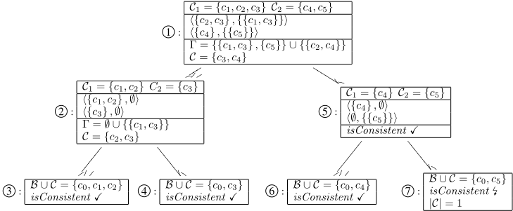
Consider a CSP consisting of six constraints {c0, ..., c5}. The constraint c0 is considered correct, i.e. B = {c0}. Let {{c0, c1, c3}, {c0, c5}, {c2, c4}} be the set of minimal conflicts. Algorithm 2 proceeds as follows (Figure 1).
Since the input CSP (B∪C) is not consistent, the algorithm enters the recursion. In the first step, FINDCONFLICTS partitions the input set (line 7) into the two subsets C1={c1,c2,c3} and C2={c4,c5} and provides them as input to the recursive calls (lines 8 and 9). In the next level of the recursion - markedwith 2 in Figure 1 - the input is found to be inconsistent (line 5) and again partitioned into two sets (line 7). In the subsequent calls, 3 and 4 , the two input sets are found to be
1 The calls in line 8 and 9 can in fact be executed in parallel.
Algorithm 2: MERGEXPLAIN(B, C)
Input: B: background theory, C: the set of possibly faulty constraints Output: Γ, a set of minimal conflicts 1 if ¬isConsistent(B) then return 'no solution'; 2 if isConsistent(B ∪ C) then return ∅; 3 〈_, Γ〉 ← FINDCONFLICTS(B, C) 4 return Γ; function FINDCONFLICTS (B, C) returns a tuple 〈C ′ , Γ〉 5 if isConsistent(B ∪ C) then return 〈C, ∅〉; 6 if |C| = 1 then return 〈∅, {C}〉; 7 Split C into disjoint, non-empty sets C1 and C2 8 〈C ′1 , Γ1〉 ← FINDCONFLICTS(B, C1) 9 〈C ′2 , Γ2〉 ← FINDCONFLICTS(B, C2) 10 Γ←Γ1 ∪Γ2; 11 while ¬isConsistent(C ′1 ∪ C ′2 ∪B) do 12 X ← GETCONFLICT(B ∪ C ′2 , C ′2 , C ′1 ) 13 CS ← X ∪ GETCONFLICT(B ∪ X, X, C ′2 ) 14 C ′1 ← C ′1 \ {α} where α ∈ X 15 Γ ← Γ ∪ {CS } 16 return 〈C ′1 ∪ C ′2 , Γ〉consistent (line 5) and, therefore, the set {c1, c2, c3} has to be analyzed using GETCONFLICT (lines 12 and 13) defined in Algorithm 1. GETCONFLICT returns the conflict {c1,c3}, which is added to Γ. Finally, FINDCONFLICTS removes c1 from the set C ′1 and returns the tuple 〈{c2,c3}, {{c1,c3}}〉 to 1 .
Next, the "right-hand" part of the initial input, the set C2={c4,c5}, is provided as input to FINDCONFLICTS 5 . Since C2 is inconsistent, it is partitioned into two sets C1={c4} and C2={c5}. The first recursive call 6 returns 〈{c4}, ∅〉 since the input in consistent. The second call 7 , in contrast, finds that the input comprises only one constraint that is inconsistent with the background theory B. Therefore, it returns 〈∅,{{c5}} in line 6. Since C ′1 ∪C ′2 = {c4}∪∅ is consistent with B, FINDCONFLICTS 5 returns 〈{c4}, {{c5}}〉 to 1 .
Finally, in 1 the set of constraints C ′1 ∪ C ′2 = {c2,c3} ∪ {c4} is found to be inconsistent with B (line 11) and GETCONFLICT is called. The method returns the conflict {c2,c4} and c2 is removed from C ′1 . The resulting set {c3,c4} is consistent and MXP returns Γ={{c1,c3}, {c5}, {c2, c4}}.
3.4 Properties of MERGEXPLAIN
Theorem 2. Given a background theory B and a set of constraints C, Algorithm 2 always terminates and returns
- 'no solution', if B is inconsistent,
- ∅, if B ∪ C is consistent, and
- a set of minimal conflicts Γ, otherwise.
Proof. In the first case, given an inconsistent background theory B, the algorithm terminates in line 1 and returns 'no solution'. In the second case, if the set B ∪ C is consistent, then no subset of C is a conflict. MXP terminates and returns ∅.
Finally, if the set B∪C is inconsistent, the algorithm enters the recursion in line 3. The function FINDCONFLICTS in each call partitions the input set C into two sets C1 and C2. The partitioning continues until either the found set of constraints C is consistent or a singleton conflict is detected. Therefore, every recursion branch ends after at most log |C| - 1 calls. Consequently, FINDCONFLICTS terminates if the conflict detection loop in lines 11-15 always terminates.
We consider two situations. If the set C ′1 ∪ C ′2 is consistent with B, the loop terminates. Otherwise, in each iteration at least one conflict in the set C ′1 ∪ C ′2 is resolved. This fact follows from Theorem 1 according to which the function GETCONFLICT in Algorithm 1 always returns a minimal conflict if the input parameter C is inconsistent with B. Since the number of conflicts is finite and in each iteration one of the conflicts in C ′1 ∪ C ′2 is resolved in line 14, the loop will terminate after a finite number of iterations. Consequently, Algorithm 2 terminates and returns a set of minimal conflicts Γ.
Corollary 1. Given a consistent background theory B and a set of inconsistent constraints C, Algorithm 2 always returns a set of minimal conflicts Γ such that there exists a diagnosis ∆i ⊆ ⋃CSi∈Γ CS i.
The proof follows from the fact that - similar to the HStree algorithm - a conflict is resolved by removing one of its elements from the set of constraints C1 in line 14. The loop in line 11 guarantees that every conflict CSi ∈ C ′1 ∪ C ′2 is hit. Consequently, FINDCONFLICTS hits every conflict in the input set C and the set of constraints {α1, . . . , αn} removed in every call of line 14 is a superset or equal to a diagnosis of the problem. The construction of at least one diagnosis from the found conflicts Γ can be done by the HS-tree algorithm.
MXP can in principle use several strategies for the resolution of conflicts in line 14. The strategy used in MXP by default is conservative and allows us to find several conflicts at once. Two additional elimination strategies can be used in line 14: (1) C ′1 ← C ′1 \ X or (2) C ′1 ← C ′1 \ CS and C ′2 ← C ′2 \ CS. These more aggressive strategies result in a smaller number of conflicts returned by MXP in each call but each call returns the results faster. However, for the latter strategies MXP might not return enough minimal conflicts for the HS-tree algorithm to compute at least one diagnosis. For instance, let {{c1, c2} , {c1, c3} , {c2, c4}} be the set of all minimal conflicts. If MXP returns Γ = {{c1, c2}}, which is one of the possible valid outputs, then the HS-tree algorithm fails to find the diagnosis as {c1, c2} must be hit twice. In this case, the HS-tree algorithm must call MXP multiple times or another algorithm for diagnosis computation must be used, e.g. [Shchekotykhin et al., 2014].
Corollary 2. Algorithm 2 is sound, i.e., every set CS ∈ Γ is a minimal conflict, and complete, i.e., given a diagnosis problem for which at least one minimal conflict exists, Algorithm 2 returns Γ ̸= ∅.
The soundness of the algorithm follows from Theorem 1, since the conflict computation of MXP uses the GETCONFLICT function of QXP. The completeness is shown as follows: Let B be a background theory and C a set of faulty constraints, i.e., B ∪ C is inconsistent. Assume MXP returns Γ = ∅, i.e., no minimal conflicts are found. However, this is impossible, since the loop in line 11 will never end. Consequently, Algorithm 2 will not terminate which contradicts our assumption. Hence, it holds that MXP is complete.
4 Evaluation
We have evaluated the efficiency of computing multiple conflicts at once with MXP using a number of different diagnosis benchmark problems. As a baseline for the comparison, we use QXP as a Theorem Prover, which returns exactly one minimal conflict at a time. Furthermore, we made measurements with a variant of MXP called PMXP in which the lines 8 and 9 are executed in parallel in two threads on a multi-core computer.
4.1 Benchmark Problems
We made experiments with different benchmark problems. First, we used the five first systems of the DX Competition (DXC) 2011 Synthetic Track. For each system, 20 scenarios are specified in which artificial faults were injected. In addition, we made experiments with a number of CSP problems from the CSP solver competition 2008 and several CSP encodings of real-world spreadsheets. The injection of faults was done in the same way as in [Jannach et al., 2015].
| System | #C | #V | #F | #D | #D | |D| | #Cf | |Cf| |
|---|---|---|---|---|---|---|---|---|
| 74182 | 21 | 28 | 4 - 5 | 30 - 300 | 139 | 4.66 | 4.9 | 3.3 |
| 74L85 | 35 | 44 | 1 - 3 | 1 - 215 | 66.4 | 3.13 | 5.9 | 8.3 |
| 74283 | 38 | 45 | 2 - 4 | 180 - 4,991 | 1,232.7 | 4.42 | 78.8 | 16.1 |
| 74181 | 67 | 79 | 3 - 6 | 10 - 3,828 | 877.8 | 4.53 | 7.8 | 10.6 |
| c432 | 162 | 196 | 2 - 5 | 1 - 6,944 | 1,069.3 | 3.38 | 15.0 | 19.8 |
In addition to these benchmark problems, we developed a diagnosis problem generator, which can be configured to generate (randomized) diagnosis problems with varying characteristics, e.g., with respect to the number of conflicts, their size, or their position in the system description SD.
4.2 Measurement Method
We implemented all algorithms in a Java-based MBD framework, which uses Choco as an underlying constraint solver, see [Jannach et al., 2015]. The experiments were conducted on a laptop computer (Intel i7, 8GB RAM). As a performance indicator we use the time needed ("wall clock") for computing one or more diagnoses. The reported running time numbers are averages of 100 runs of each problem setting that were done to avoid random effects. We furthermore randomly shuffled the ordering of the constraints in each run to avoid effects that might be caused by a certain positioning of the conflicts in SD. For the evaluation of MXP we used the most aggressive elimination strategy (2) as described in Section 3.4.
Since MXP can return more than one conflict at a time, it is expected to be particularly useful when the problem is to find a set of n first (leading) diagnoses, e.g., in the context of applying MBD to software debugging [Jannach and Schmitz, 2014; Shchekotykhin et al., 2012]. We therefore report the results for the tasks "find-one-diagnosis" (as an extreme case) and "find-n-diagnoses". When the task is to find all diagnoses, the performance of MXP is similar to that of QXP as all existing conflicts have to be determined 2 .
4.3 Results
DXC Benchmark Problems Table 1 shows the characteristics of the analyzed and CSP-encoded DXC benchmark problems. Since we consider multiple scenarios per system, the number of faults and the corresponding diagnoses can vary strongly across the experiment runs.
Table 2 shows the observed performance gains when using MXP instead of QXP in terms of absolute numbers (ms) and the relative improvement. For the problem of finding the first 5 diagnoses (QXP-5/MXP-5), the observed improvements range from 15% up to 45%. For the extreme case of finding one single diagnosis, even slightly stronger improvements can be observed. The improvements when searching for, e.g., the first 10 diagnoses are similar for cases in which significantly more than 10 diagnoses actually exist.
2 "Direct encodings" are typically more efficient than the HS-tree algorithm when the problem is to find one single diagnosis. A comparison with such approaches is however beyond the scope of our work, as we are interested in problem settings in which the HS-tree algorithm is favorable and no assumptions about the underlying reasoner should be made.
| System | QXP-5 [ms] | MXP-5 Improv. | QXP-1 [ms] | MXP-1 Improv. |
|---|---|---|---|---|
| 74182 | 17.0 | 19% | 17.0 | 19% |
| 74L85 | 20.9 | 15% | 16.1 | 19% |
| 74283 | 61.2 | 29% | 53.8 | 32% |
| 74181 | 691.8 | 45% | 637.0 | 47% |
| c432 | 707.5 | 25% | 503.9 | 37% |
| Scenario | #C | #V | #F | #D | |D| | #Cf | |Cf| |
|---|---|---|---|---|---|---|---|
| c8 | 523 | 239 | 8 | 4 | 6.25 | 7 | 1.6 |
| costasArray-13 | 87 | 88 | 2 | >5 | 3.6 | >565 | 45.6 |
| domino-100-100 | 100 | 100 | 3 | 81 | 2 | 2 | 15 |
| graceful-K3-P2 | 60 | 15 | 4 | >117 | 2.94 | >12 | 29.2 |
| mknap-1-5 | 7 | 39 | 1 | 2 | 1 | 1 | 2 |
| queens-8 | 28 | 8 | 15 | 9 | 10.9 | 15 | 2.8 |
| hospital payment | 38 | 75 | 4 | 40 | 4 | 4 | 3 |
| profit calculation | 28 | 140 | 5 | 42 | 4.25 | 11 | 9 |
| course planning | 457 | 583 | 2 | 3024 | 2 | 2 | 55.5 |
| preservation model | 701 | 803 | 1 | 22 | 1 | 1 | 22 |
| revenue calculation | 93 | 154 | 4 | 1452 | 3 | 3 | 15.7 |
Constraint Problems / Spreadsheets The characteristics for the next set of benchmark problems (six CSP competition instances, five CSP-encoded real-world spreadsheets with injected faults [Jannach et al., 2015]) are shown in Table 3.
The results for determining the five first minimal diagnoses are shown in Table 4 3 . Again, performance improvements of up to 54% can be observed. The obtained improvements vary quite strongly across the different problem instances: the higher the complexity of the underlying problem, the stronger are the improvements achieved with our new method. Only in the two cases in which only one single conflict exists (see Table 3), the performance can slightly degrade as MXP performs an additional check if further conflicts among the remaining constraints exist.
Systematically Generated MBD Problems To be able to systematically analyze which factors potentially influence the obtained performance improvements, we developed an MBD problem generator in which we could vary (i) the overall number of COMPS, (ii) the number of conflicts and their average size (and as a consequence the number of diagnoses), and (iii) the position of the conflicts in the database. We considered the last aspect because the performance of QXP and MXP can largely depend on this aspect 4 . If, e.g., there is only one conflict and the conflict is represented by the two "leftmost" elements in SD, QXP's divide-and-conquer strategy will be able to rule out most other elements very fast.
3 The results for finding one diagnosis follow the same trend.
| Scenario | QXP | MXP | |
|---|---|---|---|
| [ms] | [ms] | Impr. | |
| c8 | 615 | 376 | 39% |
| costasArray-13 | 1,379,842 | 629,366 | 54% |
| domino-100-100 | 417 | 389 | 7% |
| graceful-K3-P2 | 1611 | 1123 | 30% |
| mknap-1-5 | 32 | 36 | -11% |
| queens-8 | 281 | 245 | 13% |
| hospital payment | 1,717 | 1,360 | 21% |
| profit calculation | 86 | 76 | 12% |
| course planning | 2,045 | 1,544 | 25% |
| preservation model | 371 | 391 | -5% |
| revenue calculation | 109 | 87 | 21% |
We evaluated the following configurations regarding the position of the conflicts (see Table 5): (a) Random: The elements of each conflict are randomly distributed across SD; (b) Left/Right: All elements of the conflict appear in exactly one half of SD; (c) LaR (Left and Right): Conflicts are both in the left and right half, but not spanning both halves; (d) Neighb.: Conflicts appear randomly across SD, but only involve "neighboring" elements.
One specific rationale of evaluating these constellations individually is that conflicts in some application domains (e.g., when debugging knowledge bases) might represent "local" inconsistencies in SD.
Since the conflicts are known in advance in this experiment, no CSP solver is needed to determine the consistency of a given set of constraints in TP. Since zero computation times are unrealistic, we added simulated consistency checking times in each call to the TP. The value of the simulated time quadratically increases with the number of constraints to be checked and is capped in the experiments at 10 milliseconds. We made additional tests with different consistency checking times to evaluate to which extent the improvements obtained with MXP depend on the complexity of an individual consistency check for the underlying problem. However, these tests did not lead to any significant differences.
Table 5 shows some of the results of this simulation. In this measurement, we also include the results of the parallelized PMXP variant. The following observations can be made.
(1) The performance of QXP strongly depends on the position of the conflicts. In the probably most realistic Random case, MXP helps to reduce the computation times around 2030%. In the constellations that are "unfortunate" for QXP, the speedups achieved with MXP can be as high as 75%. When QXP is "lucky" and all conflicts are clustered in the left part of SD, some improvements or light deteriorations can be observed for MXP. The latter two situations (all conflicts are clustered in one half) are actually quite improbable but help us better understand which factors influence the performance.
4 We assume a splitting strategy in which the elements are simply split in half in the middle with no particular ordering of the elements.
| #Cp | #Cf | |Cf| | Cf Pos. | QXP [ms] | MXP Impr. | PMXP Impr. |
| 50 | 5 | 2 | Random | 351 | 27% | 30% |
| 50 | 5 | 2 | Left | 161 | 6% | 10% |
| 50 | 5 | 2 | Right | 481 | 69% | 70% |
| 50 | 5 | 2 | LaR | 293 | 51% | 57% |
| 50 | 5 | 2 | Neighb. | 261 | 54% | 58% |
| 100 | 5 | 2 | Random | 417 | 33% | 35% |
| 100 | 5 | 2 | Left | 181 | 14% | 17% |
| 100 | 5 | 2 | Right | 622 | 75% | 76% |
| 100 | 5 | 2 | LaR | 351 | 58% | 63% |
| 100 | 5 | 2 | Neighb. | 314 | 62% | 65% |
| 50 | 15 | 4 | Random | 2,300 | 22% | 20% |
| 50 | 15 | 4 | Left | 452 | -8% | -4% |
| 50 | 15 | 4 | Right | 1,850 | 72% | 73% |
| 50 | 15 | 4 | LaR | 3,596 | 22% | 18% |
| 50 | 15 | 4 | Neighb. | 166,335 | 43% | 43% |
- When comparing the results of the first two blocks in the table, it can be seen that the improvements achieved with MXP are stronger when there are more components in SD and more time is needed for performing the individual consistency checks. This is in line with the results of the other experiments.
(3) Parallelization can help to obtain modest additional improvements. The strongest improvements are observed for the LaR configuration, which is intuitive as PMXP by design explores the left and right halves independently in parallel. Note that in the experiments with the DXC and the CSP benchmark problems, in most cases we could not observe runtime improvements through parallelization. This is caused by two facts. First, the consistency checking times are often on average below 1 ms, which means that the relative overhead of starting a new thread can be comparably high. Second, the used CSP solver causes some additional overheads and thread synchronization when used in multiple threads in parallel.
5 RelatedWork
In [Junker, 2004b], Junker informally sketches a possible extension of QXP to be able to compute multiple "preferred explanations" in the context of Preference-Based Search (PBS). The general goal of Junker's approach is partially similar to our work and the proposed extended version of QXP could in theory be used during the HS-tree construction as well.
Technically, Junker proposes to set a choice point whenever a constraint ci is found to be consistent with a partial relaxation during search and thereby look for (a) branches that lead to conflicts not containing ci and (b) branches leading to conflicts in which the removal of ci leads to a solution.
Unfortunately, it is not fully clear from the informal sketch in [Junker, 2004b] where the mentioned choice point should be set. If applied in line 5 of Algorithm 1, conflicts are only found in the left-most inconsistent partition. The method would then return only a small subset of all conflicts MERGEXPLAIN would return. If the split is done for every ci consistent with a partial relaxation during PBS, the resulting diagnosis algorithm corresponds to the binary BHS-tree method [Lin and Jiang, 2003], which according to the experiments in [Pill et al., 2011] is not generally favorable over HS-Tree algorithms, in particular when we are searching for a limited set of diagnoses.
From the algorithm design, note that QXP applies a constructive conflict computation procedure prior to partitioning, whereas MXP does the partitioning first - thereby removing multiple constraints at a time - and then uses a divide-andconquer conflict detection approach. Finally, our method can, depending on the configuration, make a guarantee about the existence of a diagnosis given the returned conflicts without the need of computing all existing conflicts.
In general, our work is related to a variety of (complete) approaches from the MBD literature which aim to find diagnoses more efficiently than with Reiter's original method. Existing works for example tried to speed up the process by exploiting existing hierarchical, tree-like or distributed structural properties of the underlying problem [Stumptner and Wotawa, 2001; Wotawa and Pill, 2013], through parallelization [Jannach et al., 2015], or by solving the dual problem [Satoh and Uno, 2005; Stern et al., 2012; Liffiton et al., 2015]. A main difference to these previous works is that we make no assumption about the underlying problem structure in our approach and leave the general HS-tree procedure unchanged. Instead, our aim is to avoid a full restart of the conflict search process when constructing a new node by looking for potentially existing additional conflicts in each call, and to thereby speedup the overall process.
Beside complete methods, a number of approximate diagnosis approaches have been proposed in the last years, which for example use stochastic and heuristic search [Li and Yunfei, 2002; Feldman et al., 2010a]. The relation of our work to these approaches is limited as we are focusing on application scenarios where the goal is to find a few first diagnoses more quickly but at the same time maintain the completeness property. Finally, for some domains, "direct" and SAT-based encodings, e.g., [Metodi et al., 2012], have shown to be very efficient to find one or a few diagnoses in recent years. Most "direct" methods are however again incomplete and require the use of additional techniques like iterative deepening if the goal is to find more than one minimal diagnosis.
The concept of conflicts plays a central role in different other reasoning contexts than Model-Based Diagnosis, e.g., explanations or dynamic backtracking. Specifically, in recent years a number of approaches were proposed in the context of the maximum satisfiability problem (MaxSAT), see [Morgado et al., 2013] for a recent survey. In these domains the conflicts are referred to as unsatisfiable cores or Minimally Unsatisfiable Subsets (MUSes); Minimal Correction Subsets (MSCes) on the other hand correspond to the concept of diagnoses in this paper. In [Davies and Bacchus, 2013] or [Ignatiev et al., 2014], for example, different algorithms were recently proposed to find one solution to the MaxSAT problem, which corresponds to the problem of finding one minimal/preferred diagnosis. Other techniques such as MARCO [Liffiton et al., 2015] aim at the enumeration of conflicts. In general, many of these algorithms use a similar divide-and-conquer principle as we do with MXP. However, such algorithms - including the ones listed above - often modify the underlying knowledge base by adding relaxation variables to clauses of a given unsatisfiable formula and then use a SAT solver to find the relaxations. This strategy roughly corresponds to the direct diagnoses approaches discussed above. MXP, in contrast, acts completely independently of the underlying knowledge representation language. Moreover, the problem-independent decomposition approach used by MXP is a novel feature which - to the best of our knowledge - is not present in the existing conflict detection techniques from the MaxSAT field. Specifically, it allows our algorithm to find multiple conflicts more efficiently because it searches for them within independent small subsets of the original knowledge base. In addition, MXP can find conflicts in knowledge bases formulated in very expressive knowledge representation languages, such as description logics, which cannot be efficiently translated to SAT, see also [Shchekotykhin et al., 2014].
6 Conclusions
We have proposed and evaluated a novel, general-purpose and non-intrusive conflict detection strategy called MERGEXPLAIN, which is capable of detecting multiple conflicts in a single call. An evaluation on various benchmark problems revealed that MERGEXPLAIN can help to significantly reduce the required computation times when applied in a Model-Based Diagnosis setting in which the goal is to find a defined number of diagnoses and in which no assumption about the underlying reasoning engine should be made.
One additional property of MERGEXPLAIN is that the union of the elements of the returned conflict sets is guaranteed to be a superset of one diagnosis of the original problem. Recent methods like the one proposed in [Shchekotykhin et al., 2014] can therefore be applied to find one minimal diagnosis quickly.
Acknowledgements
This work was supported by the Carinthian Science Fund (KWF) contract KWF-3520/26767/38701, the Austrian Science Fund (FWF) and the German Research Foundation (DFG) under contract numbers I 2144 N-15 and JA 2095/4-1 (Project "Debugging of Spreadsheet Programs").
@inproceedings{ijcai2015p454,
  title     = {MergeXplain: Fast Computation of Multiple Conflicts for Diagnosis},
  author    = {Shchekotykhin, Kostyantyn M. and Jannach, Dietmar and Schmitz, Thomas},
  booktitle = {Proceedings of the Twenty-Fourth International Joint Conference on
               Artificial Intelligence, {IJCAI-15}},
  publisher = {International Joint Conferences on Artificial Intelligence},
  editor    = {Qiang Yang and Michael Wooldridge},
  pages     = {3221--3227},
  year      = {2015},
  month     = {7},
  note      = {Special Track on Knowledge Representation and Reasoning},
  url       = {https://ijcai.org/proceedings/2015/454},
}
TY - CPAPER TI - MergeXplain: Fast Computation of Multiple Conflicts for Diagnosis AU - Shchekotykhin, Kostyantyn M. AU - Jannach, Dietmar AU - Schmitz, Thomas T2 - Proceedings of the Twenty-Fourth International Joint Conference on Artificial Intelligence, IJCAI-15 PB - International Joint Conferences on Artificial Intelligence PY - 2015 SP - 3221 EP - 3227 UR - https://ijcai.org/proceedings/2015/454 ER -Copied
Machine-readable versions of this paper, for tools and AI agents:





