
Sampling with Minimum Sum of Squared Similarities for Nystrom-Based Large Scale Spectral Clustering
Proceedings of the Twenty-Fourth International Joint Conference on Artificial Intelligence. Main Track. Pages 2313-2318.
© 2015 International Joint Conferences on Artificial Intelligence
Abstract
The Nystrom method provides an efficient sampling approach for large scale clustering problems, by generating a low-rank matrix approximation. However, existing sampling methods are limited by accuracy and computing time. This paper proposes an improved Nystrom-based clustering algorithm with a new sampling procedure, Minimum Sum of Squared Similarities (MSSS). Experiments on synthetic and real data sets show that the proposed sampling performs with higher accuracy than existing algorithms, applied to Nystrom-based spectral clustering problems. Furthermore, we provide a theoretical analysis that allows us to define the upper bound of the Frobenius norm error of the MSSS.
- [Azam and Viktor, 2013] Nadia Farhanaz Azam and Herna L Viktor. Spectral clustering: An explorative study of prox- imity measures. Springer, 2013.
- [Belabbas and Wolfe, 2009] Mohamed-Ali Belabbas and Patrick J Wolfe. Spectral methods in machine learning and new strategies for very large datasets. Proceedings of the National Academy of Sciences, 106(2):369-374, 2009.
- [Chen and Cai, 2011] Xinlei Chen and Deng Cai. Large scale spectral clustering with landmark-based representa- tion. In Proceedings of the Twenty-Fifth AAAI Conference on Artificial Intelligence, AAAI 2011, San Francisco, Cal- ifornia, USA, August 7-11, 2011, 2011.
- [Chen et al., 2011] Wen-Yen Chen, Yangqiu Song, Hongjie Bai, Chih-Jen Lin, and Edward Y Chang. Parallel spec- tral clustering in distributed systems. Pattern Analysis and Machine Intelligence, IEEE Transactions on, 33(3):568- 586, 2011.
- [Cohen et al., 2014] Michael B Cohen, Yin Tat Lee, Cameron Musco, Christopher Musco, Richard Peng, and Aaron Sidford. Uniform sampling for matrix approxima- tion. arXiv preprint arXiv:1408.5099, 2014.
- [Drineas and Mahoney, 2005] Petros Drineas and Michael W Mahoney. On the nyström method for approximating a gram matrix for improved kernel-based learning. The Journal of Machine Learning Research, 6:2153-2175, 2005.
- [Drineas et al., 2006] Petros Drineas, Ravi Kannan, and Michael W Mahoney. Fast monte carlo algorithms for ma- [Fu, 2014] Zhouyu Fu. Optimal landmark selection for nys- trm approximation. In ChuKiong Loo, KeemSiah Yap, KokWai Wong, Andrew Teoh, and Kaizhu Huang, editors, Neural Information Processing, volume 8835 of Lecture Notes in Computer Science, pages 311-318. Springer In- ternational Publishing, 2014.
- [Gowda and Sznajder, 2010] M Seetharama Gowda and Ro- man Sznajder. Schur complements, schur determinantal and haynsworth inertia formulas in euclidean jordan alge- bras. Linear Algebra and Its Applications, 432(6):1553- 1559, 2010.
- [Higham et al., 2007] Desmond J Higham, Gabriela Kalna, and Milla Kibble. Spectral clustering and its use in bioin- formatics. Journal of computational and applied mathe- matics, 204(1):25-37, 2007.
- [Kong et al., 2011] Tengteng Kong, Ye Tian, and Hong Shen. A fast incremental spectral clustering for large data sets. In Parallel and Distributed Computing, Applications and Technologies (PDCAT), 2011 12th International Con- ference on, pages 1-5. IEEE, 2011.
- [Kumar et al., 2009a] Sanjiv Kumar, Mehryar Mohri, and Ameet Talwalkar. Ensemble nystrom method. In Advances in Neural Information Processing Systems, pages 1060- 1068, 2009.
- [Kumar et al., 2009b] Sanjiv Kumar, Mehryar Mohri, and Ameet Talwalkar. On sampling-based approximate spec- tral decomposition. In Proceedings of the 26th Annual In- ternational Conference on Machine Learning, pages 553- 560. ACM, 2009.
- [Shinnou and Sasaki, 2008] Hiroyuki Shinnou and Minoru Sasaki. Spectral clustering for a large data set by reduc- ing the similarity matrix size. In LREC, 2008.
- [Sloan, 1981] Ian H Sloan. Quadrature methods for integral equations of the second kind over infinite intervals. Math- ematics of computation, 36(154):511-523, 1981.
- [Von Luxburg, 2007] Ulrike Von Luxburg. A tutorial on spectral clustering. Statistics and computing, 17(4):395- 416, 2007.
- [Wang et al., 2014] Minchao Wang, Wu Zhang, Wang Ding, Dongbo Dai, Huiran Zhang, Hao Xie, Luonan Chen, Yike Guo, and Jiang Xie. Parallel clustering algorithm for large- scale biological data sets. PloS one, 9(4):e91315, 2014.
- [Williams and Seeger, 2001] Christopher Williams and Matthias Seeger. Using the nyström method to speed up kernel machines. In Proceedings of the 14th Annual Conference on Neural Information Processing Systems, number EPFL-CONF-161322, pages 682-688, 2001.
- [Zeng et al., 2014] Zhicheng Zeng, Ming Zhu, Hong Yu, and Honglian Ma. Minimum similarity sampling scheme for nyström based spectral clustering on large scale high- dimensional data. In Modern Advances in Applied Intelli- gence, pages 260-269. Springer, 2014.
- [Zhang and You, 2011] Xianchao Zhang and Quanzeng You. Clusterability analysis and incremental sampling for nyström extension based spectral clustering. In Data Min- ing (ICDM), 2011 IEEE 11th International Conference on, pages 942-951. IEEE, 2011.
- [Zhang et al., 2008] Kai Zhang, Ivor W Tsang, and James T Kwok. Improved nyström low-rank approximation and error analysis. In Proceedings of the 25th international conference on Machine learning, pages 1232-1239. ACM, 2008.
References were extracted automatically from the PDF and may contain errors.
Full text extracted automatically from the PDF; figures, tables and equations may differ. The PDF is the version of record.
1 Introduction
The amount of large-scale data around us is increasing in size very quickly. Clustering those data with respect to certain features using computational approaches would help us interpret them in a timely manner. Hence, development of clustering algorithms is an active field of research [Kong et al., 2011].
In recent years, spectral clustering has become increasingly popular, often outperforming alternative approaches on a range of datasets [Chen and Cai, 2011]. However, spectral clustering has limited applicability to large-scale problems, due to its computational time complexity. To address this computational challenge, a common approach is to use a lowrank matrix approximation [Zhang and You, 2011], [Chen and Cai, 2011]. The Nystr¨om method is one such technique used in a number of machine learning problems [Fowlkes et al., 2004], [Williams and Seeger, 2001]. The method works by first sampling a set of m landmark points from n instances, with m ≪ n, to formulate an approximation for the eigendecomposition of the full dataset using the sampled data.
The most important step of the Nystr¨om method is sampling, because different sampled landmark points give different approximations of the original matrix. Uniform sampling without replacement is the most used approach for this purpose [Fowlkes et al., 2004], [Cohen et al., 2014], where every point has the same probability of being included in the sample. Alternatively, sampling can be performed using local or global properties of the data distribution. Different versions of non-uniform sampling have recently been suggested. For example, in [Zeng et al., 2014] authors proposed an algorithm that considers the similarity between the sample set and the rest of the data points to select the landmark points. Similarly, [Zhang and You, 2011] proposed an algorithm, where points with the smallest variance between the sampled points and the rest of the data are selected as landmark points.
In this paper, we propose "Minimum Sum of Squared Similarities" (MSSS), an algorithm for incremental sampling in Nystr¨om based-spectral clustering. MSSS considers both variance and similarity in its sampling data, increasing the speed of the clustering on large datasets. The algorithm starts sampling with a fixed number of initial landmark points and selects new landmark points one by one, such that the sum of the squared similarities between the previously selected points and the new point is minimized. We also discuss its upper bound on the Frobenius norm error.
2 RelatedWork
Derived from spectral graph theory [Von Luxburg, 2007], spectral clustering has a wide range of applicability, such as in community detection [Azam and Viktor, 2013], image segmentation [Fowlkes et al., 2004] and clustering of microarray data [Higham et al., 2007].
To apply spectral clustering to large datasets, recent efforts have been concentrating on solving issues around algorithm scalability [Zeng et al., 2014], such as on reducing the time cost of eigen-decomposition of a Laplacian matrix (see 3.1) through parallel computations [Chen et al., 2011], [Wang et al., 2014]. Another approach is to use dimension reduction by Nystr¨om approximation [Williams and Seeger, 2001], a method originally designed for numerical solution of integral equations [Sloan, 1981].
Recently, due to their demonstrated effectiveness, Nystr¨om approximation-based machine learning algorithms are gaining popularity [Fu, 2014]. However the performance of the approach is highly dependent on proper subsampling of the input data to include some landmark points, points that capture the inherent complexity and variability of the full dataset. To address this, different sampling methods have been proposed, some as simple as random sampling (RS) [Fowlkes et al., 2004], [Cohen et al., 2014]. However, although it is straightforward to implement, RS makes an implicit assumption that clusters have an equiprobable distribution, which may be a limiting assumption for certain datasets [Fowlkes et al., 2004].
Two proposed alternatives use diagonal sampling [Drineas and Mahoney, 2005] and column-norm sampling [Drineas et al., 2006] algorithms, and are very effective. However, they are shown to perform poorly in various test cases in comparison to RS [Kumar et al., 2009b].
In [Belabbas and Wolfe, 2009] the authors developed a weighted sampling (WS) approach using the determinant of the kernel matrix to select landmark points, where the probability of choosing a new landmark point was in proportion to the determinant of the similarity matrix between landmark points. They analyzed the Nystr¨om reconstruction error using the Schur complement [Gowda and Sznajder, 2010], concluding that the larger the determinant, the smaller the error. Although the work provides a solid theoretical basis for measuring the error levels in Nystr¨om approximation, a main drawback of the algorithm provided is in its time complexity.
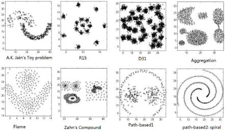
Assuming that the potential clusters are convex, [Zhang et al., 2008] introduced k-means based sampling (KS) algorithm, as a means to select points near k-means centroids as landmark points. Similarly, [Shinnou and Sasaki, 2008] also pre-processed the data using k-means clustering, to select a committee of data points near centroids. Although the latter method does not explicitly state the convexity assumption, both methods perform poorly for non-convex clusters and when clusters are grouped in certain configurations, such as some of the test datasets shown in Figure 1.
In [Zhang and You, 2011], the authors proposed an incremental sampling (IS) algorithm that first randomly samples two points from a dataset, to compute a similarity matrix between the sampled points and the remaining points. The algorithm picks the point with the smallest variance, and then iteratively repeats the process until a desired number of landmarks is reached. While promising, [Zeng et al., 2014] showed that IS performs poorly on high-dimensional data, as the variance of the Euclidean distance tends to zero. In such cases IS may pick inappropriate landmark points for dimension reduction, hence for successful clustering.
The authors in [Zeng et al., 2014] studied how the similarity between the sample set and non-sample set influences the approximation error, and proposed minimum similarity sampling (SS) for high-dimensional space clustering. However, their result depends on the dimensionality of the dataset: SS outperforms IS on high-dimensional data, but not on low dimensional data.
To address the problems raised in [Zeng et al., 2014] and [Zhang and You, 2011], we propose a new sampling algorithm, MSSS, which approximately maximizes the determinant of the reduced similarity matrix that represents the mutual similarities between sampled data points. We demonstrate the performance of MSSS in comparison to leading sampling methods using synthetic benchmark datasets, as well as a University of California, Irvine (UCI) Machine Learning Repository dataset.
3 Key Notion
3.1 Spectral clustering
Spectral clustering algorithms employ the first k eigenvectors of a Laplacian matrix to guide clustering. Loosely following the notation in [Von Luxburg, 2007], this can be outlined as follows.
Algorithm 1 Spectral Clustering Algorithm
- 1: Input: Affinity matrix S ∈ Rn×n , number of clusters to construct, k
- 2: Output: Clusters c1, ..., ck
- 3: Compute the Laplacian matrix P = D - S ; where D is an n × n diagonal matrix defined by Dii = ∑nj=1 Sij
- 4: Compute k eigenvectors u1, ..., uk corresponding to the largest k eigenvalues of the generalized eigenproblem Pu = λDu; and let Z ∈ Rn×k be the matrix containing the vectors u1, ..., uk.
- 5: Cluster y1, ..., yn by k-means algorithm into clusters c1, ..., ck; with yi corresponding to the i-th row of Z.
Here, S is the symmetric affinity matrix constructed using the cosine similarity between each pairs of data points.
By analyzing the spectrum of the Laplacian matrix constructed over all data entries, the original data can be compressed into a smaller number of representative points using the Nystr ¨om approximation described below.
3.2 Nystr¨om Sampling
The Nystr ¨om sampling method was originally designed to approximate the solutions of integral equations of the form:
where x, y ∈ R, φ(x) represents the eigenfunction, and sim(x, y) denotes the similarity between x and y.
If we consider m landmark data points L = l1, l2, ..., lm from a given dataset X = x1, x2, ..., xn with xi ∈ Rn and m ≪ n, then for any given point x in X, Nystr¨om method formulates
where ˆ φ(x) is an approximation to the exact eigenfunction, and ˆλ is the corresponding approximate eigenvalue. Note that, Eq.2 cannot be solved directly, as both ˆ φ(x) and ˆλ are unknown.
If we denote the similarity matrix between the landmark points by ˜ S with ˜ sij = sim(li, lj), and substitute x with li in Eq.2, we can write it in matrix form,
where ˆΦ = [ˆ φ1 ˆ φ2... ˆ φm] are the eigenvectors of ˜ S and ˆΛ = diag{ˆλ1, ˆλ2, . . . , ˆλm} is a diagonal matrix of the corresponding approximate eigenvalues.
For an unsampled point x, the j-th eigenfunction at x can be approximated by
With the equation above, the eigenvector for any given point x can be approximated through the eigenvectors of the landmark points L [Belabbas and Wolfe, 2009].
The same idea can be applied to extend the solution of a reduced matrix eigenvalue problem, to approximate the eigenvectors of a similarity matrix. Specifically, one may approximate k eigenvectors of S by decomposing and then extending a k × k principal sub-matrix of S.
First, let S be partitioned as
with A ∈ Rk×k .
Now, define spectral decompositions S = UΛU T and A = UAΛAU TA ; the Nystr¨om extension then provides an approximation for k eigenvectors in
where the approximations of ˜ U ≈ U and ˜Λ ≈ Λ may then be composed, yielding an approximation ˜ S ≈ S according to
We call ˜ S the Nystr¨om approximation to S.
We note from Eq.6 that the main computational load to calculate this approximation is centred around the principal sub-matrix A of dimension k < n, and hence the Nystr¨om extension provides a practical scalability for the spectral decomposition, hence for the spectral clustering problem.
4 Proposition
Before we present our approach, let us consider two toy examples to motivate the proposed algorithm.
Example 1. Assume that in a given dataset X = {x1, x2, ..., xn} the data points belong to four clusters. In the ideal case of zero inter-cluster similarities, when three landmark points are selected, the similarity matrix would be ˜ S = I3 where Ia is the a×a identity matrix with a = 3. Similarly, for a fourth landmark point xi, we would ideally have ˜ S∪{xi} = I4, implying that the new landmark point is again not at all similar to the precedent landmarks points.
Suppose, however, that we have to choose between two non-ideal landmark points, x1 and x2, such that
and
It was shown in [Zhang and You, 2011] that the larger the determinant of the reduced dimension similarity matrix, the smaller the error of the Nystr¨om approximation. Hence, in this case, one should pick x1 over x2, because det( ˜ S∪{x1}) is larger than det(˜ S∪{x2}).
However, the search for an optimum landmark point involves repeated computation of determinants, which has a time complexity of O(n3 ). Our motivation is to reduce this to O(mn) by considering the sum of squared similarities between a landmark candidate and the preceding landmark data points.
In effect, by this approach we consider both the variance and the sum of the similarities between the new and preceding landmark data points, as proposed by [Zeng et al., 2014] and [Zhang and You, 2011], respectively, since by definition
where b is the similarity vector between a new (mth ) landmark point and the preceding (m-1) landmarks, and var(b) is the variance of b.
In this example, this will allow us to pick x1 over x2, while the sum of similarities would not be able to distinguish between the two choices. The variance method would similarly pick x1 over x2.
Example 2. Expanding on the above example, let us now consider a third candidate for the new landmark, x3, such that
In this case, again x1 is preferable over x3, but this time the variance method will not be able to pick between x1 and x3, while sum of similarities and sum of squared similarities would both prefer x1, as they should.
4.1 Theoretical analysis
Next, following the formalism of [Zhang and You, 2011] we show that, under certain assumptions, selecting landmarks incrementally in a way that minimizes the sum of the squared similarities between the new and the precedent landmark points would maximize the determinant of the landmark similarity matrix.
Theorem 1. For a given dataset X = {x1, x2, . . . , xn}, let S be a real n × n, symmetric positive definite matrix, where its entries sαβ = sim(xα, xβ) describe the similarity (in [0, 1]) between xα and xβ, with sαα = 1. Let ˜ S be an optimum (m1)st order Nystr¨om approximation of S, such that ˜ S ≃ I. Denote the landmark data points that constitute this Nystr¨om approximation with ˜X = {˜x1, ˜x2, . . . , ˜xm-1}. Then, for two data points xp and xq in X but not in ˜X, if
then
Therefore, the optimum new landmark data point ˜xm that minimizes ∑i<m sim2 (˜xm, ˜xi) approximately maximizes det( ˜ S∪{˜xm}).
Proof. First, consider the augmented Nystr¨om approximation, with
where b = [b1, ..., bm-1]⊤ is the vector of similarities between new landmark ˜xm and the preceding landmarks ˜xi, i.e., bi = sim(˜xi, ˜xm) for i = 1, . . . ,m- 1.
To take the determinant of this augmented matrix, one can consider two levels of co-factor expansions over column m then by rowm-1, to give
where M<im>,<(m-1)j> is the minor < (m - 1)j > of M<im>, which in turn is the minor < im > of ˜ S∪{˜xm}, and ˜ S/i is a matrix obtained by deleting the rows and columns i ∈ 1, ...,m- 1 of the matrix ˜ S∪{˜xm}.
Note that, because ˜ S ≃ I, all determinants of the second order cofactors will be negligible, i.e.,det(M<im>,<(m-1)j>) ≃ 0, and the double summation in the second line of Eq.9 will drop.
Next, due to the constructive nature of the theorem, we will have ˜ S/i ≃ I for all i ∈ 1, ...,m- 1. Thus, we can write
for some ϵ > 0, which puts the second term on the right hand side of Eq.9 in some δ > 0 neighbourhood of ∑m-1 i=1 b2i , where δ < ϵ ∑m-1 i=1 b2i .
Finally, this gives us,
Hence, minimizing ∑m-1 i=1 b2i approximately maximizes det( ˜ S∪{˜xm}).
4.2 Minimum Sum of Squared Similarities
Our algorithm is directly deduced from Theorem 1, where rather than finding a new landmark point that maximizes the determinant, we find a point that minimizes the sum of squared similarities (MSSS). The MSSS algorithm initially randomly chooses two points from the dataset X. It then computes the sum of similarities between the sampled points and a subset, T, selected randomly from the remaining data points. The point with the smallest sum of squared similarities is then picked as the next landmark data point. The procedure is repeated until a total of m landmark points are picked.
Algorithm 2 The Minimum Sum of Squared Similarities Algorithm
γ: size of the subsampled set from the remaining data, in
- 1: Input: X = {x1, x2, ..., xn}: dataset m: number of landmark data points percentage
- 2: Output: ˜ S ∈ Rm×m: similarity matrix between landmark points
- 3: Initialize ˜ S = I0
- 4: For (i=0 to i<2) do
- 5: ˜ xi = Random(X)
- 6: ˜ S := ˜ S∪xi
- 7: ˜X := ˜X ∪ {˜ xi}
- 8: End For
- 9: While i <mdo
- 10: T = Random(X\{ ˜X}, γ)
- 11: Find ˜ xi = argminx∈T ∑j<i-1 sim2 (x, ˜ xj )
- 12: ˜ S := ˜ S∪˜ xi
- 13: ˜X := ˜X ∪ {˜ xi}
- 14: EndWhile
Theorem 2. For a dataset X = {x1, x2, ..., xn}, define the following positive definite similarity matrices:
- S: the n × n similarity matrix for the overall dataset with a maximum diagonal entry Smax;
- ˜ Sl: a similarity matrix with l landmark point selected randomly fromX;
- ˜ Sm: a similarity matrix with m landmark point selected using MSSS, with m ≤ l ≤ n; and
- Sm: the best rank-m approximation of S.
Then with some probability 1 - p or more, we can write
Proof. Using the above notation, let us introduce some facts.
Fact 1 [Belabbas and Wolfe, 2009] Let λ1 ≤ ... ≤ λn be the eigenvalues of the similarity matrix S. Then
Fact 2 [Kumar et al., 2009a] With some probability 1-p or higher, we can write the following inequality:
Then, adding both sides of Eq.11 and Eq.12, noting that ∑ni=m+1 ≥ ∑ni=l+1 , and using the Triangle inequality
5 Evaluation
We tested MSSS with two subsampling percentages, γ = 0 and 10, (MSSS and MSSS-10, respectively), and compared its performance to the results of three state-of-the-art approaches described in Section 2: random sampling (RS), kmeans sampling (KS) [Zhang et al., 2008] and minimum similarity sampling (SS) [Zeng et al., 2014]. Note that, we did not compare our algorithm to WS and IS, since it was shown earlier that SS performs better than WS and IS [Zeng et al., 2014].
We required each algorithm to sample 1%, 2%,..,10% of the data as landmark points, which are used by Nystr¨ombased spectral clustering methods to cluster the datasets.
Because sampling algorithms are sensitive to the datasets used, and clustering algorithms contain a degree of randomness, we used various benchmark datasets, and repeated our evaluations 1000 times. We measured the clustering quality of each algorithm using their average accuracy across these tests, also recording their standard deviations.
5.1 Clustering Synthetic Data
We evaluated algorithms on eight commonly used synthetic datasets 1 with different shapes (Figure 1), instances and number of clusters (Table 1). We note that, on these datasets, all tested algorithms have better performance than the baseline of random sampling.
Table 2 reports the average accuracy of each algorithm, along with their standard deviations across 1000 tests. As expected, the accuracies depend on the dataset. For example, the accuracy of all algorithms in A.K Jain's Toy problem and PathBased1 datasets stay in the range of 50%- 60%, while going as high as over 90% for the R15 and D31 datasets. We can say from this observation that the A.K Jain's Toy problem and PathBased1 datasets present difficulties to Nystr¨om method-based spectral clustering.
In the eight datasets, we see that overall MSSS algorithms perform better than the baseline random sampling. MSSS
1 http://cs.joensuu.fi/sipu/datasets/
| Dataset | Instances | Attributes | Classes |
|---|---|---|---|
| Synthetic Datasets | |||
| A.K Jain's Toy problem | 373 | 2 | 2 |
| R15 | 600 | 2 | 15 |
| D31 | 3100 | 2 | 31 |
| Aggregation | 788 | 2 | 7 |
| Flame | 240 | 2 | 2 |
| Zahn's Compound | 399 | 2 | 6 |
| Pathbased1 | 300 | 2 | 3 |
| Pathbased2:Spiral | 312 | 2 | 3 |
| UCI Datasets | |||
| Iris | 150 | 4 | 3 |
| Wine | 178 | 13 | 3 |
| Glass | 214 | 9 | 7 |
| Breast | 699 | 9 | 2 |
| Wdbc | 569 | 32 | 2 |
| Haberman | 306 | 3 | 2 |
| DUMD | 259 | 5 | 4 |
gave the best results in three datasets and MSSS-10 gave the best results in two datasets, indicating that the MSSS method offers a flexible approach, and that tuning the γ parameter for specific datasets might help for its optimum performance.
The results of the SS algorithm show overall better performance compared to KS and RS sampling. SS also gave the best performance on the R15 dataset, which has a uniform density distribution. When the density distribution is not uniform though MSSS gave higher performance than SS.
5.2 Clustering Real Data
We also compared the performance of the four sampling methods using data from University of California, Irvine (UCI) Machine Learning Repository 2 . We randomly chose seven datasets: Iris, Wine, Glass, Breast, Wdbc, Haberman and Data User Modeling Dataset (DUMD). A brief summary of the datasets is listed in Table 1.
The clustering accuracy results on the UCI datasets are shown in Table 2. The results show that MSSS provided better clustering than the other algorithms on five datasets. Ranking the algorithms with respect to their mean accuracies, we note that the top three performing algorithms were MSSS, MSSS-10 and SS, in that order. Results on the UCI dataset recapitulate our observation on synthetic data that γ in our algorithm can be tuned according to the dataset to yield better performance.
2 https://archive.ics.uci.edu/ml/datasets.html
| Table 2: Accuracy on Datasets | |||||
|---|---|---|---|---|---|
| MSSS | MSSS-10 | SS | RS | KS | |
| Synthetic Datasets | |||||
| A.K Jain's Toy problem R15 | 61.06±0.63 91.53±0.85 94.79±0.14 | 61.06±0.63 90.46±0.80 94.81±0.13 | 61.06±0.63 91.73±0.78 94.80±0.14 | 61.06±0.63 89.72±1.20 95.07±0.30 | 53.79±0.68 89.71±1.27 95.07±0.29 |
| D31 Aggregation | 78.88±0.98 | 79.03±0.98 | 78.90±0.92 | 74.73±1.18 | 74.51±1.30 |
| Flame | 73.69±8.17 | 73.70±8.17 | 73.69±8.17 | 73.69±8.17 | 70.91±6.40 |
| Zahn's Compound | 71.52±1.98 | 70.35±2.08 | 71.51±1.85 | 65.73±3.39 | 65.69±3.67 |
| PathBased1 | 62.71±4.89 | 58.49±7.15 | 61.86±5.50 | 57.32±4.77 | 56.21±4.25 |
| Pathbased2:Spiral | 72.40±4.34 | 72.27±4.46 | 72.38±4.06 | 71.50±4.84 | 66.94±5.20 |
| UCI Datasets | |||||
| Iris | 69.06±4.30 | 68.74±4.46 | 68.76±4.37 | 75.16±6.70 | 75.86±7.66 |
| Wine | 59.71±4.71 | 60.37±4.81 | 60.36±4.67 | 59.59±4.83 | 60.17±5.19 |
| Glass | 72.71±4.01 | 72.41±4.04 | 72.10±4.01 | 72.51±4.16 | 71.36±2.46 |
| Breast | 62.46±4.09 | 62.50±4.00 | 62.71±4.01 | 58.64±3.48 | 58.75±3.50 |
| Wdbc | 50.38±0.27 | 50.37±0.27 | 50.37±0.27 | 50.37±0.27 | 50.09±0.27 |
| Haberman | 55.33±1.46 | 55.22±1.44 | 55.30±1.47 | 55.10±1.39 | 55.19±1.37 |
| DUMD | 58.97±2.57 | 59.08±2.40 | 59.07±2.81 | 57.87±3.01 | 57.56±3.22 |
5.3 Comparison on Computation Time
To compare the computational time of the tested sampling algorithms, we measured the average run times for each algorithm over 1000 replicates (Table 3). Overall, we observed that all the tested algorithms have a higher computational time than RS, and that KS algorithm consumed much more time compared to other algorithms. We speculate that the poor time performance of the KS algorithm is due to the fact that it calculates k-means clusters - a computationally expensive process. The other algorithms had similar computational times. Hence we conclude that the accuracy improvement in MSSS is achieved with comparable computational time with respect to the state-of-the-art sampling algorithms.
6 Conclusion
In this paper, we introduced a new sampling algorithm, MSSS, for Nystr¨om method-based spectral clustering. The new algorithm is scalable; it can handle large-scale data with computational times comparable to the state-of-the-art. Through theoretical analyses, we provided an upper bound to the matrix approximation error for the algorithm. In benchmarking experiments we demonstrated the competitive performance of MSSS over the current state-of-the-art.
Intriguing as these results are though, we note that the second best algorithm on every dataset, be it synthetic or real, was always within one standard deviation away from the top performing algorithm. This implies that achieving performance improvement in this problem domain is becoming increasingly difficult. Yet, the MSSS algorithm demonstrates a marginal but consistent advantage over the state-of-the art. Further, the new algorithm comes with an important parameter that can be tuned for better performance over various datasets, promising added gains if it can be optimized over any given dataset, hence paving the way for future research.
MSSS is implemented in java, and its source code is available from: www.bcgsc.ca/platform/bioinfo/software/msss
7 Acknowledgments
The authors thank the funding organizations, Genome Canada, British Columbia Cancer Foundation, and Genome British Columbia for their support of this work. We also thank Dr. Victoria Stuart for her critical reading of the draft manuscript.
@inproceedings{ijcai2015p327,
  title     = {Sampling with Minimum Sum of Squared Similarities for Nystrom-Based Large Scale Spectral Clustering},
  author    = {Bouneffouf, Djallel and Birol, Inanç},
  booktitle = {Proceedings of the Twenty-Fourth International Joint Conference on
               Artificial Intelligence, {IJCAI-15}},
  publisher = {International Joint Conferences on Artificial Intelligence},
  editor    = {Qiang Yang and Michael Wooldridge},
  pages     = {2313--2318},
  year      = {2015},
  month     = {7},
  note      = {Main Track},
  url       = {https://ijcai.org/proceedings/2015/327},
}
TY - CPAPER TI - Sampling with Minimum Sum of Squared Similarities for Nystrom-Based Large Scale Spectral Clustering AU - Bouneffouf, Djallel AU - Birol, Inanç T2 - Proceedings of the Twenty-Fourth International Joint Conference on Artificial Intelligence, IJCAI-15 PB - International Joint Conferences on Artificial Intelligence PY - 2015 SP - 2313 EP - 2318 UR - https://ijcai.org/proceedings/2015/327 ER -Copied
Machine-readable versions of this paper, for tools and AI agents:





