
Scalable Graph Hashing with Feature Transformation
Proceedings of the Twenty-Fourth International Joint Conference on Artificial Intelligence. Main Track. Pages 2248-2253.
© 2015 International Joint Conferences on Artificial Intelligence
Abstract
Hashing has been widely used for approximate nearest neighbor (ANN) search in big data applications because of its low storage cost and fast retrieval speed. The goal of hashing is to map the data points from the original space into a binary-code space where the similarity (neighborhood structure) in the original space is preserved. By directly exploiting the similarity to guide the hashing code learning procedure, graph hashing has attracted much attention. However, most existing graph hashing methods cannot achieve satisfactory performance in real applications due to the high complexity for graph modeling. In this paper, we propose a novel method, called scalable graph hashing with feature transformation (SGH), for large-scale graph hashing. Through feature transformation, we can effectively approximate the whole graph without explicitly computing the similarity graph matrix, based on which a sequential learning method is proposed to learn the hash functions in a bit-wise manner. Experiments on two datasets with one million data points show that our SGH method can outperform the state-of-the-art methods in terms of both accuracy and scalability.
- [Andoni and Indyk, 2008] Alexandr Andoni and Piotr Indyk. Near-optimal hashing algorithms for approximate nearest neighbor in high dimensions. Communications on ACM, 51(1):117-122, 2008.
- [Andoni, 2009] Alexandr Andoni. Nearest Neighbor Search: The Old, The New, and The Impossible. PhD thesis, Mas- sachusetts Institute of Technology, 2009.
- [Datar et al., 2004] Mayur Datar, Nicole Immorlica, Piotr Indyk, and Vahab S. Mirrokni. Locality-sensitive hash- ing scheme based on p-stable distributions. In Proceed- ings of the Annual Symposium on Computational Geome- try, pages 253-262, 2004.
- [Gionis et al., 1999] Aristides Gionis, Piotr Indyk, and Ra- jeev Motwani. Similarity search in high dimensions via hashing. In Proceedings of the International Conference on Very Large Data Bases, pages 518-529, 1999.
- [Gong and Lazebnik, 2011] Yunchao Gong and Svetlana Lazebnik. Iterative quantization: A procrustean approach to learning binary codes. In Proceedings of the IEEE Conference on Computer Vision and Pattern Recognition, pages 817-824, 2011.
- [Huiskes et al., 2010] Mark J. Huiskes, B. Thomee, and Michael S. Lew. New trends and ideas in visual concept detection: The mir flickr retrieval evaluation initiative. In Proceedings of the ACM International Conference on Mul- timedia Information Retrieval, pages 527-536, 2010.
- [Indyk and Motwani, 1998] Piotr Indyk and Rajeev Mot- wani. Approximate nearest neighbors: Towards remov- ing the curse of dimensionality. In Proceedings of the Annual ACM Symposium on Theory of Computing, pages 604-613, 1998.
- [Kong and Li, 2012] Weihao Kong and Wu-Jun Li. Isotropic hashing. In Proceedings of the Advances in Neural Infor- mation Processing Systems, pages 1655-1663, 2012.
- [Kulis and Darrell, 2009] Brian Kulis and Trevor Darrell. Learning to hash with binary reconstructive embeddings. In Proceedings of the Advances in Neural Information Processing Systems, pages 1042-1050, 2009.
- [Kulis and Grauman, 2009] Brian Kulis and Kristen Grau- man. Kernelized locality-sensitive hashing for scalable image search. In Proceedings of the IEEE International Conference on Computer Vision, pages 2130-2137, 2009.
- [Lin et al., 2014] Guosheng Lin, Chunhua Shen, Qinfeng Shi, Anton van den Hengel, and David Suter. Fast su- pervised hashing with decision trees for high-dimensional data. In Proceedings of the IEEE Conference on Computer Vision and Pattern Recognition, pages 1971-1978, 2014.
- [Liu et al., 2011] Wei Liu, Jun Wang, Sanjiv Kumar, and Shih-Fu Chang. Hashing with graphs. In Proceedings of the International Conference on Machine Learning, 2011.
- [Liu et al., 2012] Wei Liu, Jun Wang, Rongrong Ji, Yu-Gang Jiang, and Shih-Fu Chang. Supervised hashing with ker- nels. In Proceedings of the IEEE Conference on Computer Vision and Pattern Recognition, pages 2074-2081, 2012.
- [Liu et al., 2014] Wei Liu, Cun Mu, Sanjiv Kumar, and Shih- Fu Chang. Discrete graph hashing. In Proceedings of the Advances in Neural Information Processing Systems, pages 3419-3427, 2014.
- [Norouzi and Fleet, 2011] Mohammad Norouzi and David J. Fleet. Minimal loss hashing for compact binary codes. In Proceedings of the International Conference on Machine Learning, pages 353-360, 2011.
- [Shrivastava and Li, 2014] Anshumali Shrivastava and Ping Li. Asymmetric lsh (alsh) for sublinear time maximum inner product search (mips). In Proceedings of the Ad- vances in Neural Information Processing Systems, pages 2321-2329, 2014.
- [Song et al., 2013] Jingkuan Song, Yang Yang, Yi Yang, Zi Huang, and Heng Tao Shen. Inter-media hashing for large-scale retrieval from heterogeneous data sources. In Proceedings of the ACM SIGMOD International Confer- ence on Management of Data, pages 785-796, 2013.
- [Wang et al., 2010a] Jun Wang, Ondrej Kumar, and Shih-Fu Chang. Semi-supervised hashing for scalable image re- trieval. In Proceedings of the IEEE Conference on Com- puter Vision and Pattern Recognition, pages 3424-3431, 2010.
- [Wang et al., 2010b] Jun Wang, Sanjiv Kumar, and Shih-Fu Chang. Sequential projection learning for hashing with compact codes. In Proceedings of the International Con- ference on Machine Learning, pages 1127-1134, 2010.
- [Weiss et al., 2008] Yair Weiss, Antonio Torralba, and Robert Fergus. Spectral hashing. In Proceedings of the Ad- vances in Neural Information Processing Systems, pages 1753-1760, 2008.
- [Xu et al., 2013] Bin Xu, Jiajun Bu, Yue Lin, Chun Chen, Xiaofei He, and Deng Cai. Harmonious hashing. In Pro- ceedings of the International Joint Conference on Artificial Intelligence, 2013.
- [Zhang and Li, 2014] Dongqing Zhang and Wu-Jun Li. Large-scale supervised multimodal hashing with seman- tic correlation maximization. In Proceedings of the AAAI Conference on Artificial Intelligence, pages 2177-2183, 2014.
- [Zhang et al., 2014] Peichao Zhang, Wei Zhang, Wu-Jun Li, and Minyi Guo. Supervised hashing with latent factor models. In Proceedings of the International ACM SIGIR Conference on Research and Development in Information Retrieval, pages 173-182, 2014.
- [Zhen and Yeung, 2012] Yi Zhen and Dit-Yan Yeung. A probabilistic model for multimodal hash function learning. In Proceedings of the ACM SIGKDD International Con- ference on Knowledge Discovery and Data Mining, pages 940-948, 2012.
- [Zhu et al., 2013] Xiaofeng Zhu, Zi Huang, Heng Tao Shen, and Xin Zhao. Linear cross-modal hashing for efficient multimedia search. In Proceedings of the ACM Interna- tional Conference on Multimedia, pages 143-152, 2013.
References were extracted automatically from the PDF and may contain errors.
Full text extracted automatically from the PDF; figures, tables and equations may differ. The PDF is the version of record.
1 Introduction
Nearest neighbor search [Andoni, 2009] plays an important role in a large variety of areas including machine learning, data mining, and information retrieval, and so on. In big data applications, it is typically time-consuming or impossible to return the exact nearest neighbors to the given queries. In fact, approximate nearest neighbors (ANN) [Indyk and Motwani, 1998; Andoni and Indyk, 2008] are enough to achieve satisfactory performance in many applications, such as the image retrieval task in search engines. Furthermore, ANN search is usually more efficient than exact nearest neighbor search to solve large-scale problems. Hence, ANN search has attracted more and more attention in this big data era [Andoni and Indyk, 2008]
Because of its low storage cost and fast retrieval speed, hashing [Andoni and Indyk, 2008; Wang et al., 2010a; Gong and Lazebnik, 2011; Zhen and Yeung, 2012; Zhu et al., 2013;
Song et al., 2013; Zhang et al., 2014; Liu et al., 2014] has been widely used for ANN search. The hashing techniques used for ANN search are usually called similarity-preserving hashing, which tries to map the data points from the original space into a binary-code Hamming space where the similarity (neighborhood structure) in the original space is preserved. More specifically, the Hamming distance between the binary codes of two points should be small if these two points are similar in the original space. Otherwise, the Hamming distance should be as large as possible. With the binary-code representation, hashing can achieve constant or sub-linear time complexity for ANN search [Gong and Lazebnik, 2011; Zhang et al., 2014]. Furthermore, hashing can also reduce the storage cost dramatically. For example, only 4GB memory is needed to store one billion data points if each point is represented as a binary code of 32 bits. Hence, hashing has become one of the most popular methods for ANN search [Gionis et al., 1999; Datar et al., 2004; Weiss et al., 2008; Kulis and Darrell, 2009; Wang et al., 2010b; Liu et al., 2011; Gong and Lazebnik, 2011; Kong and Li, 2012; Liu et al., 2012; Xu et al., 2013; Zhang et al., 2014; Lin et al., 2014; Liu et al., 2014].
Compared with traditional data-independent hashing methods like locality sensitive hashing (LSH) [Gionis et al., 1999; Datar et al., 2004] which do not use any data for training, data-dependent hashing methods, which are also called learning to hash (LH) methods, can achieve comparable or better accuracy with shorter codes by learning hash functions from training data [Gong and Lazebnik, 2011; Liu et al., 2012; Zhang et al., 2014; Liu et al., 2014]. Hence, LH methods have become more popular than data-independent methods [Wang et al., 2010b; Gong and Lazebnik, 2011; Liu et al., 2012; Zhang et al., 2014; Lin et al., 2014; Liu et al., 2014].
Existing LH methods can be divided into two main categories [Gong and Lazebnik, 2011; Liu et al., 2012; Zhang et al., 2014]: unsupervised hashing and supervised hashing methods. Unsupervised hashing tries to preserve the Euclidean similarity between the attributes of training points, while supervised hashing [Norouzi and Fleet, 2011; Zhang et al., 2014; Lin et al., 2014] tries to preserve the semantic similarity constructed from the semantic labels of the training points. Although supervised hashing methods have demonstrated promising performance in some applications with semantic labels, it is time-consuming or impossible to get semantic labels in many real applications. Hence, we can only perform unsupervised hashing for these cases, which is also the focus of this paper.
Representative unsupervised hashing methods include spectral hashing (SH) [Weiss et al., 2008], binary reconstructive embeddings (BRE) [Kulis and Darrell, 2009], principal component analysis based hashing (PCAH) [Gong and Lazebnik, 2011], iterative quantization (ITQ) [Gong and Lazebnik, 2011], anchor graph hashing (AGH) [Liu et al., 2011], isotropic hashing (IsoHash) [Kong and Li, 2012], and discrete graph hashing (DGH) [Liu et al., 2014]. Among these methods, SH, BRE, AGH and DGH are graph hashing methods. By directly exploiting the similarity (neighborhood structure) to guide the hashing code learning procedure, the objective of graph hashing exactly matches the goal of similarity-preserving hashing. Hence, graph hashing should be expected to achieve better performance than other nongraph based hashing methods if the learning algorithms are effective enough.
However, most existing graph hashing methods cannot achieve satisfactory performance in real applications due to the high complexity for graph modeling. More specifically, the similarity typically reflects the pairwise relationship between two points. The memory cost for storing all the pairwise similarities is O(n2 ), where n is the number of training points. The time complexity for directly computing all the pairwise similarities is also O(n2 ). Besides these costs to compute and store the similarity graph, almost all methods will introduce extra computation and memory cost during the learning procedure. Hence, it is memory-consuming and time-consuming or even intractable to learn from the whole similarity graph for large-scale datasets which are typical in hashing applications. Existing methods have to adopt approximation or subsampling methods for graph hashing on large-scale datasets. For example, SH uses an eigenfunction solution of 1-D Laplacian for approximation by assuming uniform data distribution, which actually loses the neighborhood structure in the data. BRE has to subsample a small subset for training even if a large-scale dataset is available. Both SH and BRE cannot achieve satisfactory performance in real applications, which has been verified by existing work [Liu et al., 2011]. Both AGH and DGH use anchor graphs to approximate the similarity graph, which successfully avoid the O(n2 ) complexity for both memory and computation cost. However, the accuracy of approximation cannot be guaranteed, which might deteriorate the accuracy of the learned codes. Furthermore, it need extra computation cost to construct the anchors, which will be proved to be timeconsuming in our experiment. Hence, although the objective is attractive, existing graph hashing methods cannot achieve satisfactory performance in real applications.
In this paper, we propose a novel method, called scalable graph hashing with feature transformation (SGH), for largescale graph hashing. The main contributions of SGH are briefly outlined as follows:
- Inspired by the asymmetric LSH (ALSH) [Shrivastava and Li, 2014], SGH adopts a feature transformation method to effectively approximate the whole graph with-
out explicitly computing the pairwise similarity graph matrix. Hence, the O(n2 ) computation cost and storage cost are avoided in SGH, which makes SGH suitable for large-scale applications.
- A sequential learning method is proposed to learn the hash functions in a bit-wise manner, which is effective because the residual caused by former bits can be complementarily captured in the following bits.
- Experiments on two datasets with one million data points show that our SGH method can outperform the state-of-the-art methods in terms of both accuracy and scalability.
The rest of this paper is organized as follows. Section 2 introduces the problem definition of this paper. We present our SGH method in Section 3. Experiments are shown in Section 4, and finally we conclude the whole paper in Section 5.
2 ProblemDefinition
2.1 Notation
We use boldface lowercase letters like v to denote vectors, and the ith element of v is denoted as vi. Boldface uppercase letters like V denote matrices. The ith row of V is denoted as Vi∗, the jth column of V is denoted as V∗j, and the (i, j)th element in V is denoted as Vij. VT is the transpose of V, and tr(V) is the trace of matrix V. ‖V‖F = √∑ij V 2 ij is the Frobenius norm, which can also be used to define the length of a vector. sgn(·) is an element-wise sign function. [u; v] denotes the concatenation of two vectors u and v. Id is an identity matrix with dimensionality d.
2.2 Graph Hashing
Assume we are given n data points X = [x1; x2; · · · ; xn]T ∈ Rn×d , where d is the dimensionality of the data points and Xi∗ = xTi . Without loss of generality, the data are assumed to be zero centered which means ∑ni=1 xi = 0. Hashing is to map each point xi into a binary code bi ∈ {-1, +1}c , where c denotes the code size (length). In general, we use c binary hash functions {hk(·)|k = 1, 2, · · · , c} to compute the binary code of xi, i.e., bi = [h1(xi), h2(xi), · · · , hc(xi)]T .
We have different metrics to measure the similarity between two points in the original space. Let Sij denote the similarity between xi and xj. One most widely used metric
is defined as: Sij = e- ‖xi-xj‖2F ρ , where ρ > 0 is a parameter. We can find that Sij ∈ (0, 1]. Hashing need to preserve the similarity in the original feature space. More specifically, the larger the similarity between xi and xj is, the smaller the Hamming distance between bi and bj will be. In other words, for any three points xi, xj and xk, if Sij < Sik, the Hamming distance between bk and bi should be smaller than that between bj and bi.
If we compute all the pairwise similarities between any two points in X, we can get a similarity graph with the graph matrix S = [Sij ]n×n ∈ Rn×n . Graph hashing tries to use all the information or part of the information in S to learn the binary codes. It's obvious that both the time complexity and storage complexity are O(n2 ) if we explicitly compute all the pairwise similarities in S, which is not acceptable in large-scale applications. Hence, as stated in the introduction, existing methods have to adopt approximation or subsampling techniques to solve it. However, they cannot achieve satisfactory performance, which motivates the work in this paper.
3 Scalable Graph Hashing with Feature Transformation
In this section, we present the details of our graph hashing method SGH, including the model, learning algorithm, and complexity analysis.
3.1 Model
The model of SGH contains two key components: the objective function and the feature transformation method.
Objective Function
The aim of SGH is to approximate the similarity matrix S by the learned hashing codes, which results in the following objective function:
where ˜ Sij = 2Sij - 1. Note that ˜ Sij ∈ (-1, 1], and the relative distance in S is kept in ˜S. We use ˜S in the objective function to keep consistent with the range of 1c bTi bj ∈ [-1, 1].
It is NP-hard to directly learn the binary codes {bl} in (1). As in kernelized locality-sensitive hashing (KLSH) [Kulis and Grauman, 2009] and supervised hashing with kernels (KSH) [Liu et al., 2012], we define the hash function for the kth bit of bi as follows:
where W ∈ Rc×m is the weight matrix, φ(xi, xj ) is a kernel function which is a RBF (Gaussian) function in our experiment, m denotes the number of kernel bases, and biask is a bias value. Our goal is to learn H(x) = {h1(x), · · · , hc(x)} to map the whole training set X to a binary matrix B ∈ {-1,+1}n×c with Bi∗ = bTi . biask is typically set to - 1n ∑ni=1 ∑mj=1 Wkjφ(xi, xj), which has the same effect as that by making the training data in the kernel space zerocentered. In fact, the above hash function can be rewritten as hk(x) = sgn(K(x)wk), where wk = WT k∗ and K(x) = [φ(x, x1) - ∑ni=1 φ(xi, x1)/n, · · · , φ(x, xm) - ∑ni=1 φ(xi, xm)/n]. Then, by substituting the H(x) into (1), we can get the objective function with the parameter W to learn:min
where K(X) ∈ Rn×m is the kernel feature matrix for all training points in X.
Feature Transformation
As stated in Section 2, both time complexity and storage complexity are O(n2 ) if we explicitly compute all the pairwise similarities in ˜S, which is obviously unscalable. Here, we propose a feature transformation method to use all the similarities without explicitly computing ˜S.
We first define P(x) and Q(x) as follows:
where we multiply a value √ 2(e2-1) eρ e- ‖x‖2F ρ to x, and then add two extra dimensions.
Then we can get:
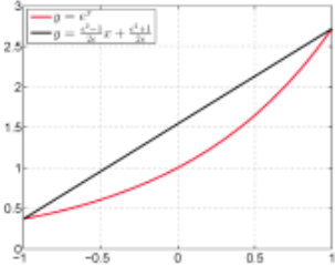
Here, we use an approximation e2-1 2e x + e2+1 2e ≈ ex , which is shown in Figure 1 when x ∈ [-1, 1]. We can find that these two functions are close to each other with x ∈ [-1, 1]. Hence, to make the approximation reasonable, we assume -1 ≤ 2ρ xTi xj ≤ 1. It is easy to prove that ρ = 2max{‖xi‖2F }ni=1 can make -1 ≤ 2ρ xTi xj ≤ 1. Actually, 2max{‖xi‖2F }ni=1 is not a tight bound of ρ. In real applications, we can also treat ρ as a hyper-parameter, and tune it with cross-validation techniques.
By using this simple feature transformation, we can derive the similarity matrix ˜S = P(X)T Q(X), where P(X) = {P(x1), · · · , P(xn)} ∈ R(d+2)×n and Q(X) = {Q(x1), · · · ,Q(xn)} ∈ R(d+2)×n . Both the time and storage complexities are still O(n2 ) if we explicitly computing ˜S = P(X)T Q(X) even if the feature transformation is adopted. However, we use only P(X) and Q(X) for computation, but do not explicitly computing ˜S in our following learning algorithm. Hence, the O(n2 ) complexity can be avoided in our method.
Please note that the feature transformation is inspired by ALSH [Shrivastava and Li, 2014], which is proposed for maximum inner product search with data-independent hashing. Different from ALSH, our SGH is for data-dependent hashing. Furthermore, the feature transformation method in SGH is different from that in ALSH.
3.2 Learning
The discrete sgn(·) function in (2) makes the problem very difficult to solve. One possible solution is to discard the discrete constraints and relax the whole H(·) function to a real-valued function, which has been adopted by many methods such as SH [Weiss et al., 2008] and AGH [Liu et al., 2011]. However, this relaxation procedure may lead to poor performance, which has been verified by existing work [Kong and Li, 2012; Zhang and Li, 2014]. Here, we design a sequential learning strategy in a bit-wise manner, where the residual caused by former bits can be complementarily captured in the following bits [Liu et al., 2012; Zhang and Li, 2014].
Assuming that we have already learned t-1 bits which are parameterized by {wi}t-1 i=1 , the residual matrix to reconstruct the similarity matrix can be computed as follows:
Then our objective function to learn the tth bit can be written as follows:
The objective function in (5) is still a NP-hard problem due to the sgn(·) function. In order to solve the problem in (5), we apply spectral relaxation [Weiss et al., 2008] and impose an orthogonality constraint to get the following formulation:
The problem in (6) can be further simplified to:
Then we reformulate the problem in (6) as follows:
Then we can obtain a generalized eigenvalue problem as follows:
If we define At = K(X)T RtK(X), then we have:
and
Equation (8) is the key component of our learning algorithm. It is easy to see that we not only implicitly include all the information of the pairwise similarity matrix ˜S for training, but also successfully avoid the high computation and storage complexity without explicitly computing ˜S.
After t iterates from 1 to c, we can learn all the W = {wi}ci=1 . Actually, the sequential learning procedure can further continue by adopting the following residual matrix:
We find that this procedure can further improve the accuracy. In our paper, we continue it for another c iterations, which achieves a good tradeoff between accuracy and speed.
The sequential learning strategy is briefly summarized in Algorithm 1. Here, γ is a very small positive number to avoid numerical problems, which is 10-6 in our experiments.
Algorithm 1 Sequential learning algorithm for SGH
Input: Feature vectors X ∈ Rn×d ; code length c; number of kernel bases m.
Output: Weight matrix W ∈ Rc×m.
Procedure
Construct P(X) and Q(X) according to (3);
Construct K(X) based on the kernel bases, which are m points randomly selected from X;
for t = 1 → c do
Solve the following generalized eigenvalue problem
̂A0 = Ac+1
Randomly permutate {1, 2, · · · , c} to generate a random index set M;
̂A0 = ̂A0 + K(X)T sgn(K(X)wˆ t )sgn(K(X)wˆ t )T K(X); Solve the following generalized eigenvalue problem
̂A0v = λZv;
Update wˆ t ←v
̂A0 = ̂A0 - K(X)T sgn(K(X)wˆ t )sgn(K(X)wˆ t )T K(X); end for
| Method | TINY-1M | MIRFLICKR-1M | ||||||||
|---|---|---|---|---|---|---|---|---|---|---|
| 32 bits | 64 bits | 96 bits | 128 bits | 256 bits | 32 bits | 64 bits | 96 bits | 128 bits | 256 bits | |
| SGH | 0.4697 | 0.5742 | 0.6299 | 0.6737 | 0.7357 | 0.4919 | 0.6041 | 0.6677 | 0.6985 | 0.7584 |
| ITQ | 0.4289 | 0.4782 | 0.4947 | 0.4986 | 0.5003 | 0.5177 | 0.5776 | 0.5999 | 0.6096 | 0.6228 |
| AGH | 0.3973 | 0.4402 | 0.4577 | 0.4654 | 0.4767 | 0.4299 | 0.4741 | 0.4911 | 0.4998 | 0.506 |
| DGH-I | 0.3974 | 0.4536 | 0.4737 | 0.4874 | 0.4969 | 0.4299 | 0.4806 | 0.5001 | 0.5111 | 0.5253 |
| DGH-R | 0.3793 | 0.4554 | 0.4871 | 0.4989 | 0.5276 | 0.4121 | 0.4776 | 0.5054 | 0.5196 | 0.5428 |
| PCAH | 0.2457 | 0.2203 | 0.2000 | 0.1836 | 0.1421 | 0.2720 | 0.2384 | 0.2141 | 0.1950 | 0.1508 |
| LSH | 0.2507 | 0.3575 | 0.4122 | 0.4529 | 0.5212 | 0.2597 | 0.3995 | 0.466 | 0.5160 | 0.6072 |
3.3 Complexity Analysis
The computation cost can be divided in two parts: initialization and the main procedure. Initialization of P(X) and Q(X), kernel initialization, and initialization of A0 and Z will cost O(dn + dmn + mn + (m2 + mn)(d + 2) + m2n). The main procedure will cost O(c(mn +m2 ) +m3 ). Typically, m, d, c will be much less than n. Hence, the time complexity of SGH is O(n) although all the n2 similarities have been used. Furthermore, the memory cost is also O(n) since the similarity matrix ˜S is not explicitly computed. Therefore, it is expected that SGH is not only accurate but also scalable.
4 Experiment
We use two datasets with one million data points for evaluation. All the experiments are conducted on a workstation with Intel (R) CPU E5-2620V2@2.1G 12 cores and 64G RAM.
4.1 Datasets
We evaluate our method on two widely used large-scale benchmark datasets: TINY-1M [Liu et al., 2014] and MIRFLICKR-1M [Huiskes et al., 2010].
The first dataset is TINY-1M which contains one million images from the 80M tiny images. Each tiny image is represented by a 384-dim GIST descriptors extracted from the original image of size 32×32.
The second dataset is MIRFLICKR-1M from LIACS Medialab at Leiden University. This dataset has one million Flickr images which are downloaded from Flickr. We extract 512 features from each image.
4.2 Evaluation Protocols and Baselines
For each dataset, we randomly select 5000 data points to construct the test (query) set and the remaining points will be used for training. The groundtruth neighbors of each query are defined as the top 2% nearest neighbors in the training set in terms of the Euclidean distance. So each query has 19900 ground truth neighbors for both datasets.
The baselines for comparison contain one dataindependent method LSH [Datar et al., 2004] and some representative unsupervised hashing methods, including two graph-based hashing methods AGH [Liu et al., 2011] and DGH [Liu et al., 2014], two linear projection based methods PCAH [Gong and Lazebnik, 2011] and ITQ [Gong and Lazebnik, 2011]. By using different initialization strategies, DGH has two variants [Liu et al., 2014], DGH-I and DGH-R, both of which are used for comparison. Please note that two other graph hashing methods SH and BRE are not adopted for comparison because existing works have shown that AGH and DGH can outperform them [Liu et al., 2014]. For kernel feature construction, we use Gaussian kernel and take 300 randomly sampled points as kernel bases for our method. We set the parameter ρ = 2 in P(X) and Q(X). For all the other baselines, we set the parameters by following the suggestions of the corresponding authors.
The Top-K precision [Liu et al., 2014] is adopted as a metric to evaluate our method and baselines. In real applications such as search engines, the users may only be interested in the top returned results given a query. Hence, the Top-K precision is a good metric for evaluation.
4.3 Accuracy
The Top-1000 precision based on the Hamming ranking results is shown in Table 1. We can see that SGH achieves the best accuracy in all the cases except on MIRFLICKR-1M with 32 bits. In particular, SGH can outperform all the other graph hashing methods in all cases. This shows that SGH is effective to capture the similarity information in the data.
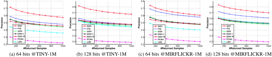
We also report the Top-K precision with other numbers of K (returned samples) in Figure 2 on two datasets with 64 bits and 128 bits. The cases with other numbers of bits are similar to these reported results, which are omitted for space saving. We can see that SGH achieves the best accuracy for different numbers of K.
| Method | 32 bits | 64 bits | 96 bits | 128 bits | 256 bits |
|---|---|---|---|---|---|
| SGH | 34.49 | 52.37 | 71.53 | 89.65 | 164.23 |
| ITQ | 31.72 | 60.62 | 89.01 | 149.18 | 322.06 |
| AGH | 18.60 + 1438.60 | 19.40 + 1438.60 | 20.08 + 1438.60 | 22.48 + 1438.60 | 25.09 + 1438.60 |
| DGH-I | 187.57 + 1438.60 | 296.99 + 1438.60 | 518.57 + 1438.60 | 924.08 + 1438.60 | 1838.30 + 1438.60 |
| DGH-R | 217.06 + 1438.60 | 360.18 + 1438.60 | 615.74 + 1438.60 | 1089.10 + 1438.60 | 2300.10 + 1438.60 |
| PCAH | 4.29 | 4.54 | 4.75 | 5.85 | 6.49 |
| LSH | 1.68 | 1.77 | 1.84 | 2.55 | 3.76 |
| Method | 32 bits | 64 bits | 96 bits | 128 bits | 256 bits |
|---|---|---|---|---|---|
| SGH | 41.51 | 59.02 | 74.86 | 97.25 | 168.35 |
| ITQ | 36.17 | 64.61 | 89.50 | 132.71 | 285.10 |
| AGH | 17.99 + 1564.86 | 18.80 + 1564.86 | 20.30 + 1564.86 | 19.87 + 1564.86 | 21.60 + 1564.86 |
| DGH-I | 85.81 + 1564.86 | 143.68 + 1564.86 | 215.41 + 1564.86 | 352.73 + 1564.86 | 739.56 + 1564.86 |
| DGH-R | 116.25 + 1564.86 | 206.24 + 1564.86 | 308.32 + 1564.86 | 517.97 + 1564.86 | 1199.44 + 1564.86 |
| PCAH | 7.65 | 7.90 | 8.47 | 9.23 | 10.42 |
| LSH | 2.44 | 2.43 | 2.71 | 3.38 | 4.21 |
4.4 Speed
We report the time consumption on two datasets in Table 2 and Table 3, respectively. Please note the "+1438.60" and "+1564.86" in the two tables denote the anchor graph constructing time in AGH and DGH. It is fair to include this anchor graph constructing time for comparison because the time of our SGH also includes all the training time. We can find that our SGH is much faster than AGH and DGH in all cases, and is faster than ITQ in most cases. LSH and PCAH are faster than SGH, but their accuracy is not satisfactory.
4.5 Sensitivity to Parameters
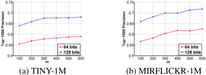
Figure 3 shows the Top-1000 precision on TINY-1M and MIRFLICKR-1M for different numbers of kernel bases (m). We can find that better accuracy can be achieved with larger m, which is consistent with our intuition. However, larger m will result in higher computation cost. Hence, in real applications, we need to choose a suitable m for tradeoff between accuracy and cost.
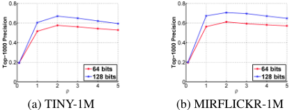
Figure 4 shows the Top-1000 precision on TINY-1M and MIRFLICKR-1M for different values of ρ. We can find that the accuracy is not sensitive to ρ when 1 ≤ ρ ≤ 5. One nice phenomenon is that our method achieves the best accuracy when ρ = 2 on both datasets.
5 Conclusion
In this paper, we have proposed a novel method, called SGH, for large-scale graph hashing. SGH is scalable by avoiding explicitly computing the similarity matrix, and simultaneously SGH can preserve the entire similarity information in the dataset. Experiments show that SGH can outperform the state-of-the-art methods in terms of both accuracy and scalability.
6 Acknowledgements
This work is supported by the NSFC (No. 61472182), and the Fundamental Research Funds for the Central Universities (No. 20620140510).
@inproceedings{ijcai2015p318,
  title     = {Scalable Graph Hashing with Feature Transformation},
  author    = {Jiang, Qing-Yuan and Li, Wu-Jun},
  booktitle = {Proceedings of the Twenty-Fourth International Joint Conference on
               Artificial Intelligence, {IJCAI-15}},
  publisher = {International Joint Conferences on Artificial Intelligence},
  editor    = {Qiang Yang and Michael Wooldridge},
  pages     = {2248--2253},
  year      = {2015},
  month     = {7},
  note      = {Main Track},
  url       = {https://ijcai.org/proceedings/2015/318},
}
TY - CPAPER TI - Scalable Graph Hashing with Feature Transformation AU - Jiang, Qing-Yuan AU - Li, Wu-Jun T2 - Proceedings of the Twenty-Fourth International Joint Conference on Artificial Intelligence, IJCAI-15 PB - International Joint Conferences on Artificial Intelligence PY - 2015 SP - 2248 EP - 2253 UR - https://ijcai.org/proceedings/2015/318 ER -Copied
Machine-readable versions of this paper, for tools and AI agents:





