
Biclustering Gene Expressions Using Factor Graphs and the Max-Sum Algorithm
Proceedings of the Twenty-Fourth International Joint Conference on Artificial Intelligence. Main Track. Pages 925-930.
© 2015 International Joint Conferences on Artificial Intelligence
Abstract
Biclustering is an intrinsically challenging and highly complex problem, particularly studied in the biology field, where the goal is to simultaneously cluster genes and samples of an expression data matrix. In this paper we present a novel approach to gene expression biclustering by providing a binary Factor Graph formulation to such problem. In more detail, we reformulate biclustering as a sequential search for single biclusters and use an efficient optimization procedure based on the Max Sum algorithm. Such approach, drastically alleviates the scaling issues of previous approaches for biclustering based on Factor Graphs obtaining significantly more accurate results on synthetic datasets. A further analysis on two real-world datasets confirms the potentials of the proposed methodology when compared to alternative state of the art methods.
- [Aji and McEliece, 2000] S.M Aji and R. J McEliece. The generalized distributive law. IEEE Tr. on Information The- ory, 46(2):325-343, 2000.
- [Badea and Tilivea, 2007] L. Badea and D. Tilivea. Stable biclustering of gene expression data with nonnegative ma- trix factorizations. In IJCAI, pages 2651-2656, 2007. IJCAI
- [Ben-Dor et al., 2003] A. Ben-Dor, B. Chor, R. Karp, and Z. Yakhini. Discovering local structure in gene expres- sion data: the order-preserving submatrix problem. J. of computational biology, 10(3-4):373-384, 2003.
- [Bicego et al., 2012] M. Bicego, P. Lovato, A. Perina, M. Fa- soli, M. Delledonne, M. Pezzotti, A. Polverari, and V. Murino. Investigating topic models' capabilities in ex- pression microarray data classification. IEEE/ACM Tr. on Comput. Biol. Bioinformatics, 9(6):1831-1836, 2012.
- [Bishop, 2006] C.M. Bishop. Pattern recognition and ma- chine learning, volume 1. springer New York, 2006.
- [Cheng and Church, 2000] Y. Cheng and G. M Church. Bi- clustering of expression data. In ISMB, p. 93-103, 2000.
- [Denitto et al., 2014] M. Denitto, A. Farinelli, G. Franco, and M. Bicego. A binary Factor Graph model for biclus- tering. In S+SSPR, pages 394-403. Springer, 2014.
- [Deodhar et al., 2009] M. Deodhar, G. Gupta, J. Ghosh, H. Cho, and I. Dhillon. A scalable framework for discov- ering coherent co-clusters in noisy data. In ICML, pages 241-248. ACM, 2009.
- [Dolnicar et al., 2012] S. Dolnicar, S. Kaiser, K. Lazarevski, and F. Leisch. Biclustering overcoming data dimensional- ity problems in market segmentation. JTR, 51(1):41-49, 2012.
- [Farinelli et al., 2011] A. Farinelli, M. Denitto, and M. Bicego. Biclustering of expression microarray data using affinity propagation. In PRIB, pages 13-24, 2011.
- [Frey and Dueck, 2007] B. Frey and D. Dueck. Cluster- ing by passing messages between data points. Science, 315:972-976, 2007.
- [Gasch et al., 2000] A. P Gasch, P. T Spellman, C. M Kao, O. Carmel-Harel, M. B Eisen, G. Storz, D. Botstein, and P. O Brown. Genomic expression programs in the response of yeast cells to environmental changes. Molecular biol- ogy of the cell, 11(12):4241-4257, 2000.
- [Hochreiter et al., 2010] S. Hochreiter, U. Bodenhofer, M. Heusel, A. Mayr, A. Mitterecker, A. Kasim, T. Khami- akova, S. Van Sanden, D. Lin, W. Talloen, et al. Fabia: factor analysis for bicluster acquisition. Bioinformatics, 26(12):1520-1527, 2010.
- [Ihmels et al., 2004] J. Ihmels, S. Bergmann, and N. Barkai. Defining transcription modules using large-scale gene ex- pression data. Bioinformatics, 20(13):1993-2003, 2004.
- [Irissappane et al., 2014] A. A Irissappane, S. Jiang, and J. Zhang. A biclustering-based approach to filter dishonest advisors in multi-criteria e-marketplaces. In Proceedings of the 2014 AAMAS, pages 1385-1386. IFAAMAS, 2014.
- [Kschischang et al., 2001] F.R. Kschischang, B.J. Frey, and H.A. Loeliger. Factor graphs and the sum-product algo- rithm. IEEE Tr. on Information Theory, 47(2):498 -519, 2001.
- [Madeira and Oliveira, 2004] S.C. Madeira and A.L. Oliveira. Biclustering algorithms for biological data analysis: a survey. IEEE Tr. on Computational Biology and Bioinformatics, 1:24-44, 2004.
- [Mukhopadhyay et al., 2014] A. Mukhopadhyay, U. Maulik, S. Bandyopadhyay, and C. A C. Coello. Survey of mul- tiobjective evolutionary algorithms for data mining: Part ii. IEEE Tr. on Evolutionary Computation, 18(1):20-35, 2014.
- [Oghabian et al., 2014] A. Oghabian, S. Kilpinen, S. Hau- taniemi, and E. Czeizler. Biclustering methods: Biolog- ical relevance and application in gene expression analysis. PloS one, 9(3):e90801, 2014.
- [Pansombut et al., 2011] T. Pansombut, W. Hendrix, Z. Ja- cob Gao, B. E Harrison, and N. F Samatova. Biclustering- driven ensemble of bayesian belief network classifiers for underdetermined problems. In IJCAI, volume 22, page 1439, 2011.
- [Prelic et al., 2006] A. Prelic, S. Bleuler, P. Zimmermann, A. Wille, P. Bhlmann, W. Gruissem, L. Hennig, L. Thiele, and E. Zitzler. Comparison of biclustering methods: A systematic comparison and evaluation of bicluster- ing methods for gene expression data. Bioinformatics, 22(9):1122-1129, 2006.
- [Rogers et al., 2005] S. Rogers, M. Girolami, C. Campbell, and R. Breitling. The latent process decomposition of cdna microarray data sets. IEEE/ACM Tr. on Comput. Biol. Bioinformatics, 2(2):143-156, 2005.
- [Sokal, 1958] Robert R Sokal. A statistical method for evaluating systematic relationships. Univ Kans Sci Bull, 38:1409-1438, 1958.
- [Tanay et al., 2002] A. Tanay, R. Sharan, and R. Shamir. Discovering statistically significant biclusters in gene ex- pression data. Bioinformatics, 18:S136-S144, 2002.
- [Truong et al., 2013] D. T. Truong, R. Battiti, and M. Brunato. A repeated local search algorithm for biclustering of gene expression data. In SIMBAD, pages 281-296. Springer, 2013.
- [Tu et al., 2011] K. Tu, X. Ouyang, D. Han, and V. Honavar. Exemplar-based robust coherent biclustering. In SDM, pages 884-895. SIAM, 2011.
- [Weiss and Freeman, 2001] Y. Weiss and W.T. Freeman. Correctness of belief propagation in gaussian graphi- cal models of arbitrary topology. Neural Computation, 13(10):2173-2200, 2001.
- [Wiberg et al., 1995] N. Wiberg, H.A. Loeliger, and R. Kot- ter. Codes and iterative decoding on general graphs. Eu- ropean Tr. on telecommunications, 6(5):513-525, 1995.
- [Yang et al., 2005] J. Yang, H. Wang, W. Wang, and P. S Yu. An improved biclustering method for analyzing gene ex- pression profiles. IJAIT, 14(05):771-789, 2005.
References were extracted automatically from the PDF and may contain errors.
Full text extracted automatically from the PDF; figures, tables and equations may differ. The PDF is the version of record.
1 Introduction
The problem of biclustering, also known as co-clustering or subspace clustering, has received an increasing attention in recent years, due to the wide range of possible applications in crucial fields such as Computational Biology and Bioinformatics [Oghabian et al., 2014; Madeira and Oliveira, 2004].
Briefly, biclustering represents a particular kind of clustering, where the goal is to "perform simultaneous row-column clustering": given a data matrix, the objective is to find sets of rows showing a coherent behavior within a certain subsets of columns. While biclustering approaches have been exploited in many different application fields [Dolnicar et al., 2012; Mukhopadhyay et al., 2014; Irissappane et al., 2014], the most important application scenario is biology [Oghabian et al., 2014; Pansombut et al., 2011; Madeira and Oliveira, 2004], in particular for the analysis of gene expression matrices [Truong et al., 2013; Badea and Tilivea, 2007]. These matrices represent the expression level of different genes in different experimental conditions, e.g. healthy/unhealthy individuals, different stages of growth and so on. In this context, the biclusters - sets of genes coherently expressed in a sets of experiments - provide priceless information: they can reveal the activation of particular biological processes, which can be involved in diseases or complex cellular operations.
Many approaches are present in the literature to solve the biclustering problem, each one characterized by different features, such as formulation, accuracy, computational complexity, descriptiveness of retrieved biclusters and so on - see the recent review in [Oghabian et al., 2014]. To face the intrinsic high computational intractability of this NP complete problem, several methods resort to heuristics, which show important limitations in terms of quality of solutions. In this paper we investigate the use of Factor Graphs to model biclustering so to combat such complexity - Factor Graphs are a class of probabilistic approaches which permit to graphically express a global function as a collection of factors (local functions) defined over subsets of variables [Kschischang et al., 2001]. Such decomposition can lead to powerful algorithms (e.g. the well known Max-Sum 1 ) which have been used to effectively solve various computational tasks (e.g. the Affinity Propagation algorithm for clustering [Frey and Dueck, 2007]). However, to derive effective solutions we have to face the dualism existing between the representation power (the more complex the model the better) and the computability of the model (the simpler the model the better): from one hand we have to derive a decomposable function, which however should be descriptive enough to capture the nature of the problem; from the other we have to deal with the model resolution, which highly depends on its topology (e.g. number of cycles for the Max-Sum algorithm).
In the biclustering context these issues are still far to be completely solved, and for this reason there are very few approaches based on Factor graphs [Farinelli et al., 2011; Tu et al., 2011; Denitto et al., 2014]. In particular, in [Farinelli et al., 2011] the clustering algorithm of Affinity Propagation [Frey and Dueck, 2007] has been adapted to the gene expression biclustering simply by performing an iterative and sequential row-column clustering. Recently [Denitto et al., 2014] extended the binary Factor Graph of Affinity Propagation with a constraint allowing to retrieve only those clusters of the matrix entries which represent true biclusters (i.e. subsets of rows and columns); this, however, results in a complex model, that can not be efficiently solved by the Max Sum algorithm (i.e. too many cycles are present [Weiss and Freeman, 2001]). Authors proposed a linear programming solution, which does not scale beyond 10x10 matrices. An alternative and interesting approach has been proposed in [Tu et al., 2011], where a more compact Factor Graph model has been derived by abandoning the binary nature of the AP Factor Graph. However, also in this case the scalability represented the main issue (the binary nature was essential in [Frey and Dueck, 2007] to derive efficient and fast routines to update the messages): actually, with the Max Sum algorithm, only a 10x10 matrix was analysed, while for larger matrices authors had to derive an approximated Max-Sum algorithm and a greedy approach.
1 Max-Sum is a message passing optimization algorithm belonging to the Generalized Distributive Law family [Aji and McEliece, 2000; Bishop, 2006; Frey and Dueck, 2007]
In this paper we take one step forward towards this direction, by proposing a novel Factor Graph approach for the gene expression biclustering problem which tries to exploit all the potential of Factor Graphs. In particular, we reformulate the biclustering problem as a sequential search for one bicluster at time 2 , then we derive a novel Factor Graph model following some of the ideas contained in [Tu et al., 2011; Denitto et al., 2014]. Crucially, the model we propose remains compact and is binary: this allows to derive an efficient optimization procedure through the Max Sum algorithm, which drastically alleviates the scaling issues of the previous approaches.
Such method has been tested on synthetic gene expression matrices of dimension 50x50, perturbed with random increasing noise. When compared with the approximated versions of [Tu et al., 2011; Denitto et al., 2014] needed to face matrices of such dimensions, the proposed approach is more accurate in identifying biclusters, thus confirming the potential of a complete exploitation of Factor Graphs in this context. Moreover, we compare our approach with previous approaches for biclustering on two gene expression datasets (yeast and breast tumor) using standard experimental protocols. Our results show that our method favourably compares with the state of the art in both data-sets.
2 RelatedWork
In the literature, the exploitation of Factor Graphs and the max-sum algorithm for gene expression biclustering is still rather limited [Denitto et al., 2014; Tu et al., 2011].
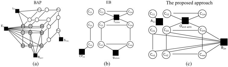
In particular, [Denitto et al., 2014] proposed an extension of the Factor Graph presented in [Frey and Dueck, 2007] for the well known Affinity Propagation clustering algorithm. The main idea of that work is to perform clustering directly on the data matrix entries, instead of clustering whole rows or columns, adding a constraint which guarantees the bicluster structure (i.e. all entries have to belong to the same subset of rows and columns, composing a sub-matrix). The clustering, as in Affinity Propagation, is based on the concept of exemplar (or prototype) and is ruled by two simple constraints: i) every point (entry) has to chose one, and only one, exemplar on the basis of a similarity criterion; ii) if a point i chooses another point j as an exemplar, j has to choose itself as an exemplar. The clusters are then composed by the points choosing the same exemplar. Another constraint has to be introduced in the model ensuring that the obtained clusters could be arranged in sub-matrices (i.e. all the entries belonging to a cluster must form a rectangular). This results in a tri-dimensional binary model where the variables encode the exemplar choices between the points. Given a data matrix with n rows and m columns the model is composed by n · m layers of n ×m variables each. This, however, results in a large and complex model (for a 10×10 matrix the model contains ten thousand variables), that can not be solved with the Max Sum algorithm. Authors proposed a linear programming solution, which however does not permit to analyse matrices larger than 10x10. The Factor Graph of this approach, which we call Biclustering Affinity Propagation (BAP), is shown in Figure 1a.
2 This represents a trick employed by many approaches in the literature [Cheng and Church, 2000; Ben-Dor et al., 2003; Hochreiter et al., 2010].
The second approach [Tu et al., 2011], which we call Exemplar-based Biclustering (EB), shares many aspects with the BAP approach: in particular biclustering is again performed by exploiting the concept of exemplars and the biclustering constraint. The main difference concerns the way the representative choices are described: in this approach the variables are not any more binary, but encode with an integer value the element chosen as exemplar. As a result, the model is more compact than the previous one - n×m variables - see Figure 1b. However they lost the binary nature of the original AP scheme, which is a key element to derive efficient and fast messages update rules for the Max-Sum algorithm [Frey and Dueck, 2007]: hence in the paper the largest analysed matrix was a 10x10 matrix, while for larger matrices authors had to derive an approximated Max-Sum algorithm and a greedy approach.
3 The proposed approach
The proposed approach starts from some of the ideas contained in [Tu et al., 2011; Denitto et al., 2014] and draws a compact and binary Factor Graph model for biclustering gene expressions. We then derive a fair approach for Max Sum messages update.
3.1 The ingredients
The model is designed on the basis of four main ingredients.
- Formulate the bisclutering problem as a repeated "Search for the largest bicluster". Many approaches in the literature faced the biclustering problem in this way [Cheng and Church, 2000; Ben-Dor et al., 2003; Hochreiter et al., 2010]: once detected, a bicluster is masked in the data matrix, e.g. by replacing it with background noise [Cheng and Church, 2000]. With this assumption, we can model the solution with a set of binary variables, one for each entry of the matrix, which indicates if that entry (point) belongs to the bicluster. We have therefore a compact set of variables (as in the EB model), which are however binary (as in the BAP model). In our model, a solution is represented by a binary matrix C indicating which points belong to the bicluster (ci,j = 1) and which do not (ci,j = 0) 3 . Since
3 With i ∈ N, set of rows, and j ∈ M set of columns.
we are looking for the largest bicluster, solutions where many ci,j set to 1 would be preferred.
- The expression level "counts". When analysing gene expressions, the most important biclusters are those related to over-expression (i.e. genes presenting higher expression level than their average). This can be directly encoded in the model by rewarding solutions which contain entries with high activation levels aij (we assume all activation levels positive). This aspect was neglected in the two previously described models, where the assignment to a bicluster was made only on the basis of the coherence.
- A bicluster is "coherent". The model should prefer solutions containing coherent entries, or, in other words, should penalize incoherent solutions. In our model, the incoherence of a bicluster is measured as the sum of the pairwise incoherences between all the points belonging to the bicluster. This differs from BAP and EB models, where only the coherence with the exemplar of the bicluster has been considered. We will see that this can lead to a more robust solutions, especially in presence of noise. To define the incoherence I(aij, atk) between two entries aij and atk, we have different possibilities, depending from which kind of bicluster we are looking for (constant-value, additive, multiplicative and so on [Madeira and Oliveira, 2004]). The most straightforward option is to simply use a constant-type incoherence, like the one employed in the BAP model:
If we are looking for additively coherent biclusters, I(aij, atk) can be defined as in [Tu et al., 2011; Cheng and Church, 2000]:
- A bicluster is a "submatrix". The model should consider only valid assignments, i.e. a sub-matrix of the data matrix: this can be expressed by enforcing that the points belonging to a bicluster have to compose a rectangle. In particular, considering every pair of rows (or columns) in the binary C matrix described above, the constraint is satisfied in two cases: i) if the rows (or columns) share the same pattern or ii) if one of the rows (or columns) is completely zero. Thanks to the simplicity of the model, the number of this constraints drastically reduces: for
the EB and the BAP models, we must insert one constraint for every couple of entries, whereas here we only have a constraint for every pair of rows (or columns) 4 .
3.2 The model
Summarizing, given a data matrix A = (aij), i ∈ N = {1..n}, j ∈ M = {1..m}, aij ≥ 0, the goal is to find a bicluster BT,K = (alr), l ∈ T, r ∈ K, which can defined as a sub-matrix of A (for T ⊆ N and K ⊆ M). The proposed model, graphically sketched in Figure 1c, is fully defined by the following components:
Variables. A set C of m× n binary variables ci,j (i ∈ N and j ∈ M), each one indicating if the entry i, j belongs (ci,j = 1) or not (ci,j = 0) to the solution.
Factors.
- Aij: one for each entry i, j, encodes the activation level provided by each entry of the data matrix, and is defined as
- Oaij,atk : one for each pair of points, encodes the "incoherence" aspect of the problem, and is defined as
- Bjk: one for each couple of rows (or columns), forces the result to be a bicluster, and is defined as
4 This reduction is even more significant in the gene expression case, where typically only few experiments are present.
Optimization Function.
with [i, t] ∈ N and [j, k] ∈ M. Besides the third part (which ensures correct solutions), we have two driving forces: from one hand, if two entries ij and tk are considered in the solution (i.e. cij = 1 and ctk = 1), their activation levels (aij and atk) are summed to the objective function, this encouraging large biclusters; from the other hand a value I(aij, atk) is subtracted, avoiding incoherent points to be part of the solution. In order to balance the strength of these two forces a parameter w has been introduced into the model.
3.3 Optimization
There are at least two big classes of resolution algorithms to solve Factor Graphs: message passing algorithms and search based algorithms. Thanks to its success in the coding theory, message-passing approaches are typically preferred [Wiberg et al., 1995]. One of the most famous message passing approaches is the max-sum algorithm, which is based on the definition of two functions - called messages - which pass information between two nodes connected by a link. The Max-Sum algorithm uses two kinds of messages:
- From factors to variables:
- From variables to factors:
where ne(·) retrieves the neighbour set of the argument.
These messages are iteratively exchanged between graph nodes until a convergence criteria is reached. The variable configuration is then obtained by summing all the incoming messages in each variable, and by assigning to such variable the value that maximizes the summation [Frey and Dueck, 2007; Bishop, 2006].
A crucial element for the practical use of Max-Sum is the derivation of efficient procedures to update the messages. Obtaining such messages update rules can be not trivial (especially for messages from functions to nodes, which contain a maximization), and it is clearly linked to the structure of the model. In our case, by exploiting the binary nature of the variables and by defining the constraint (which limits the feasible variable configurations), we obtained the following messages 5 :
5 In particular, our model is composed by three different types of factors, thus six kind of messages should be derived (three in each direction); however, after some simplifications, all the MaxSum algorithm can be implemented using four messages.
- from the variable ci,j to the function Oaij,atk :
- from the variable ci,j to the function Bi,k:
- from the function Oaij,atk to the variable ci,j:
- from the function Bi,k to the variable ci,j:
with
Different convergence criteria can be used, here we stop the procedure when the variables configuration does not change for 100 consecutive iterations.
3.4 Analysis
Complexity: given a data matrix with n rows and m columns, the model has a space complexity of O(n2m2 ) (because there are n2m2 Oaij ,atk factors) while the time complexity is ruled by the O(n2 ) required by the ηk ij message update rule 6 .
Scheduling: the messages are updated in parallel using the messages retrieved in the previous iteration.
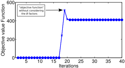
Convergence: one of the main feature of the method is that not only an explicit form for all the messages has been retrieved, but also, the messages are robust and stable. As we can see from Figure 2 the messages drive the objective function to rapidly reach its final value, which means that the variables configuration is quickly set to its convergence state.
4 Experimental Evaluation
The proposed approach has been evaluated using two sets of synthetic datasets and two real gene expression matrices.
6 The other messages require: i) ψtk ij → O(n), ii) βk ij → O(n), iii) σtk ij →O(1)
4.1 Synthetic Experiments
The two synthetic benchmarks are created to simulate gene expression matrices containing a single bicluster. In the first dataset the implanted biclusters are constant valued bicluster (we call this "Constant Bicluster Benchmark"), while in the second dataset additively coherent biclusters were used (we call this "Evolutionary Bicluster Benchmark").
In both cases, each matrix has been generated using the following procedure: i) we generate a 50 × 50 matrix containing random values uniformly distributed between 0 and 1; ii) we insert a constant valued (or additively coherent valued) bicluster, whose dimension was 25% of the matrix size, the bicluster was inserted in a random position; iii) finally, the entire matrix has been perturbed with Gaussian noise. The standard deviation of the Gaussian noise is a percentage of the difference between the mean of the entries belonging to the bicluster and the mean of the background. 5 different noise levels (i.e. percentages) were used, ranging from 0 (no noise) to 0.2 (high noise). For each noise level, 15 matrices have been generated, resulting in a total of 75 matrices.
The quality of the retrieved biclusters have been assessed using two standard indices, also employed in [Tu et al., 2011]: i) purity: percentage of points retrieved by the algorithms which actually belong to the real bicluster; ii) inverse purity: percentage of points belonging to the true bicluster which have been retrieved by the algorithms. Calling C the bicluster found by the algorithm and L the ground truth, the indices are calculated as follows:
The proposed approach has been compared with the two FGbased methods described in Section 2, namely the Biclustering Affinity Propagation (BAP) [Denitto et al., 2014] and the Exemplar-based biclustering (EB) [Tu et al., 2011]. In both cases, since the dimension of the analysed matrices is far beyond the computational capabilities of the original versions, we employed the approximated versions. In particular, for the BAP we employed the heuristic aggregation methodology proposed in [Denitto et al., 2014], which groups results obtained on smaller matrices (here we used 5x5 matrices, with no overlap). Regarding similarity, we employed the negative of the Euclidean distance (as proposed in [Denitto et al., 2014]) for the Constant Bicluster Benchmark, whereas for the Evolutionary Bicluster Benchmark we adopted the negative of eq. (1), so to deal with additively coherent biclusters.
For the EB, we employed the greedy version given in [Tu et al., 2011] 7 . Since this algorithm provides a pool of biclusters as solution, for a fair comparison all parameters have been varied inside the suggested range 8 using ten equally spaced values and only the bicluster which maximizes the product of purity and inverse purity has been considered (the product allows us to choose fairly on the basis of both indexes). The same strategy has been employed to set the coherence weight (w) for our approach (in this case, only 8 values were considered).
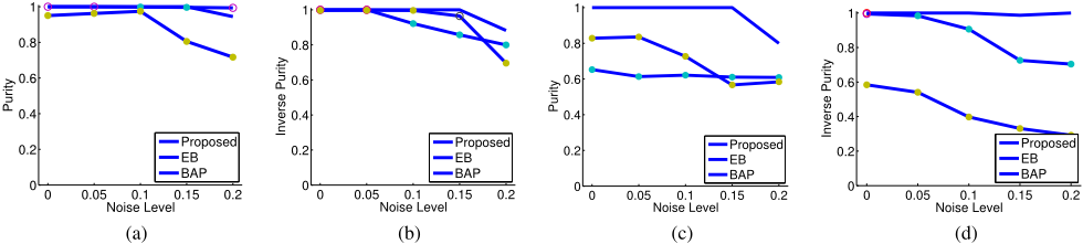
The results for the Constant and Evolutionary Bicluster benchmarks are shown in Figure 3, where purity (3a,3c) and inverse purity (3b,3d) are displayed for the different methods, while varying the noise level. Each point represents the average over the 15 runs of the given noise level. In the plot, a full marker indicates that the difference between the considered method and the proposed approach is statistically significant 9 .
7 The code can be downloaded from http://sist.shanghaitech.edu.cn/faculty/tukw/sdm11code.zip
8 Parameter ranges are described in the code documentation.
9 We performed a t-test for each noise level (on the result of the 15 matrices),we set the significance level to 5%.
The results evidently show that the proposed approach significantly outperforms the two approximated BAP and EB methods, especially when the level of noise increases, thus confirming the need of more robust optimization strategies in complex highly noisy situations. Concerning the other two methods, it is important to note that the BAP algorithm performs well only on the Constant Bicluster Benchmark: probably, employing eq. (1) as similarity is not enough to appropriately identify evolutionary biclusters. This is probably due to the fact that if two points are on the same row (or columns) the function (1) returns zero a coherence value, increasing the chance of taking part to the solution. The EB algorithm seems to be more robust, even if suffering more in case of additive coherent biclusters. Probably, in this case, assuming that a bicluster is fully described by a single entry (the exemplar) is too reductive, especially when the complexity increases due to the presence of high noise.
4.2 Gene Expression data
The algorithm has been tested on two real gene expression datasets: the Yeast dataset [Gasch et al., 2000] and the Breast tumor data [Oghabian et al., 2014].
Even if our method scales better than the other Factor Graph models, the analysis of such matrices is not possible (the algorithm runs out of memory, in particular for what concerns the memory required by η and σ messages). To combat this, the original algorithm has been executed on different portions of the matrices; successively an aggregation method to join the biclusters has been employed. More in detail, the proposed approach has been applied several times on randomly extracted submatrices (involving 10 rows and all the columns, with no overlap). The obtained biclusters have been then grouped together using Affinity Propagation, defining as similarity criterion the number of columns shared by two biclusters (the more the better). Finally, the groups of biclusters have been validated by looking at the Factor Graph objective function (2). In particular, for each group of biclusters, such function has been evaluated on the matrix composed by the rows and the columns of the biclusters belonging to it: if the objective function is positive (i.e. our algorithm could have put them togheter), the group is maintained, and the final bicluster is obtained by merging rows and columns of all its biclusters 10 .
For both datasets, the obtained biclusters are evaluated by analyzing the Gene Ontology terms of the genes belonging to the same bicluster. Briefly, Gene Ontology describes gene products in terms of their associated biological processes, cellular components and molecular functions in a speciesindependent manner, thus representing a widely used and powerful approach to validate information extracted from gene expression biclusters. The Gene Ontology analysis have been then performed on these sets through the FuncAssociate 11 web-service using five significance levels. As stated in [Tu et al., 2011], "the biclustering result is assigned a Gene Ontology enrichment score for each significance levels that corresponds to the percentage of gene sets that are enriched with respect to at least one GO annotation".
10 To retrieve different biclusters the methodology has been repeated varying the initial set of sub-matrices.
11 http://llama.mshri.on.ca/funcassociate/
| Significance Level (%) | 5 | 1 | 0.5 | 0.1 | 0.01 |
|---|---|---|---|---|---|
| Cheng&Church (%) | ∼80 | ∼70 | ∼70 | ∼55 | ∼45 |
| ROCC(%) | ∼98 | ∼98 | ∼98 | ∼98 | ∼98 |
| Bimax(%) | 100 | 100 | 100 | 100 | 100 |
| EB(%) | 100 | 100 | 100 | 100 | 100 |
| Proposed (%) | 100 | 100 | 100 | 100 | 100 |
| FABIA | ISA | Hiearc. | SAMBA | FLOC | Proposed |
| 55% | 63% | 70% | 73% | 85% | 87.5% |
For what concern the Yeast dataset, in order to be comparable with the results in [Tu et al., 2011], only the first 100 biggest biclusters (with a maximum overlap degree of 25 percent) have been considered as part of the solution. In Table 1 we reported percentages obtained with our algorithm, for different significance levels, together with other state of the art results taken from [Tu et al., 2011]. As can be seen from the table, the proposed approach compares very well with other alternatives on this dataset.
For what concern the Breast dataset, as it is commonly done in relevant literature [Rogers et al., 2005; Bicego et al., 2012] we preliminary employed variance-based gene selection to reduce the dimensionality of the data matrix; then we applied our approach, using the validation protocol adopted in [Oghabian et al., 2014]: only the first 40 largest biclusters have been considered as part of the solution, for which the Gene Ontology significance index has been evaluated with a significance level of 5%. Results are reported in Table 2, and compared with all the state of the art methods analysed in [Oghabian et al., 2014]: as can be seen from the table, our method sets a novel state of the art on this dataset.
5 Conclusions
In this paper we proposed a novel Factor Graph based approach to address the biclustering problem for gene expression data. In particular, we faced the problem by searching iteratively one bicluster at a time. We proposed a binary and compact Factor Graph based on the analysis of the data matrix entries. The model has been then solved exploiting the max-sum algorithm: i) deriving an approach to efficiently update messages and ii) analyzing the method for what concern space and time complexity. The empirical evaluation showed that our approach significantly outperforms previous stateof-the-art methods on both synthetic datasets and real data, demonstrating its practical significance.
@inproceedings{ijcai2015p135,
  title     = {Biclustering Gene Expressions Using Factor Graphs and the Max-Sum Algorithm},
  author    = {Denitto, Matteo and Farinelli, Alessandro and Bicego, Manuele},
  booktitle = {Proceedings of the Twenty-Fourth International Joint Conference on
               Artificial Intelligence, {IJCAI-15}},
  publisher = {International Joint Conferences on Artificial Intelligence},
  editor    = {Qiang Yang and Michael Wooldridge},
  pages     = {925--930},
  year      = {2015},
  month     = {7},
  note      = {Main Track},
  url       = {https://ijcai.org/proceedings/2015/135},
}
TY - CPAPER TI - Biclustering Gene Expressions Using Factor Graphs and the Max-Sum Algorithm AU - Denitto, Matteo AU - Farinelli, Alessandro AU - Bicego, Manuele T2 - Proceedings of the Twenty-Fourth International Joint Conference on Artificial Intelligence, IJCAI-15 PB - International Joint Conferences on Artificial Intelligence PY - 2015 SP - 925 EP - 930 UR - https://ijcai.org/proceedings/2015/135 ER -Copied
Machine-readable versions of this paper, for tools and AI agents:





