The Complexity of MAP Inference in Bayesian Networks Specified Through Logical Languages

1 Introduction

What is the complexity of finding most probable explanations in Bayesian networks? Conventional wisdom says that such a search is an NP-complete problem; if the network has polytree structure, matters improve as the problem then lies in P. But suppose the network is specified so that every probability distribution is a deterministic function, except for a few selected marginal probabilities. Complexity should clearly depend on which deterministic functions can be used when specifying probabilities. So, the question is: what is the complexity of finding most probable explanations (MPE) and maximum a posteriori (MAP) configurations, as parameterized by the language that is allowed in specifying the deterministic functions? This is the question we explore in this paper. More precisely, we look at deterministic functions that are specified through logical formulas. In doing so, we are inspired by previous work that focused solely on inference problems [Cozman and Mauá, 2015].

It is surprising that even for propositional languages we find our question to produce a nuanced set of results. We spend most of this paper considering combinations of conjunction, disjunction, and negation, and we are able to pinpoint the crucial role of disjunction in complexity jumps.

Even though most existing results on complexity of Bayesian networks assume that probability distributions are given as tables of rational numbers [de Campos, 2011; Kwisthout, 2014; Kwisthout et al., 2010; Pearl, 1988; Shimony and Domshlak, 2003], in practical situations the specification language does matter. For instance, one may have algorithmic gains by employing Noisy-OR gates and the like [Heckerman, 1989; Pearl, 1988], by resorting to supermodular functions Fabio G. Cozman Universidade de São Paulo São Paulo, Brazil fgcozman@usp.br

[Nemhauser et al., 1978; Greig et al., 1989] or to relational languages that make symmetries explicit [Getoor et al., 2007; Poole, 2003], or even by considering regular structures [Weller and Jebara, 2013]. By parameterizing the complexity of finding MPE and MAP by specification language, we seek to understand this interplay between expressivity and computational cost. We show that restrictions on language can sometimes bypass the effect of graph topology and can lead to tractable inferences even in networks of high treewidth. On the other hand, we show that MAP inference is intractable even for some very simple (sub Boolean) languages.

We start with some necessary background in Section 2, and then examine the complexity of MPE and MAP inferences in propositional languages (Section 3). Section 4 examines template (relational) languages. Section 5 concludes the paper.

2 MPE andMAP, parameterized by language

A Bayesian network consists of a directed acyclic graph whose nodes are random variables X1, . . . ,Xn and a collection of conditional probability distributions P(Xi|pa(Xi)), one distribution for each variable/node in the graph. Roughly speaking, the treewidth of a graph measures its tree-likeness, with a minimum treewidth of one characterizing trees. The inferential complexity of Bayesian networks has been shown to be strongly tied to the treewidth when the probability distributions are specified using tables of rationals [Kwisthout, 2014; Kwisthout et al., 2010]. On the other hand, there is an extensive literature on exploiting local structure such as determinism, symmetry and parameter sharing to speed up inference [Nemhauser et al., 1978; Heckerman, 1989; Greig et al., 1989; Poole, 2003; Weller and Jebara, 2013].

In order to circumvent the treewidth barrier, and formalize the inferential complexity in terms of local structure, Cozman and Mauá [Cozman and Mauá, 2015] recently proposed using Bayesian networks over Boolean variables (i.e., taking values {0, 1}) whose conditional probability distributions P(Xi|pa(Xi)) are deterministic functions specified as logical equivalences Xi ⇔ φi(X1, . . . , Xi-1, Xi+1, . . . , Xn), where φi is a well-formed formula in some (fixed) language L. 1 They showed that such networks can represent any network (by augmenting the model), and that new classes of Bayesian networks with tractable marginal inference can be found by restricting the language in which conditional probabilities are specified.

1 Following [Cozman and Mauá, 2015], we use variables and their corresponding propositions interchangeably.

Given a Bayesian network over variables X1, . . . ,Xn, a set of so-called MAP variables M ⊆ {X1, . . . , Xn} and an event E formed by a conjunction of assignments Xe = xe, where Xe is a variable not in M, the maximum a posteriori configuration problem is to compute

The decision variant of the problem (denoted by MAP) is to decide whether (1) exceeds a given rational number. When M and E span all variables, the problem is known as the most probable explanation problem (denoted by MPE). We refer to E as the evidence. When variables are Boolean, we call an assignment Xe = 1 a positive evidence, and an assignment Xe = 0 a negative evidence.

The aim of this work is to investigate the complexity of MAP and MPE inferences parameterized by the language in which conditional probabilities are specified. We denote by Prop(O1,O2, . . . ) the set of propositional well-formed formulas with propositions and Boolean operators O1, O2, . . . . For instance, Prop(∧, ¬) is the set propositional sentences with conjunction and negation (hence all propositional sentences). We denote by (¬) the negation operator that can only be applied to root variables (i.e., variables with no parents).

For instance, consider the celebrated QMR-DT network (meaning "Quick Medical Reference, Decision-Theoretic" network) [Shwe et al., 1991]. This is a large network with a bipartite graph where root nodes are "diseases" and non-root nodes are "findings", all of them represented by Boolean variables. There are about 600 diseases in QMR-DT, each one of them associated with a marginal probability assessment, and about 4000 findings, each one of them associated with a Noisy-OR gate. That is, QMR-DT is clearly a network specified within the framework described, using Prop(∧, ∨) as specification language. In fact, QMR-DT is a perfect example of a network that has very large treewidth (there are cliques with more than 150 variables in efficient triangulations), and that can be handled by smart exploitation of the specification language [Heckerman, 1989].

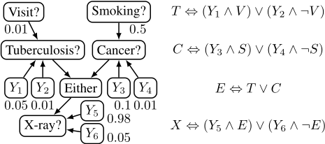
Now consider another example, where the point is to mention fact that any Bayesian network can be specified with Prop(∧, ¬). Figure 1 shows a small fragment of the popular Asia network [Lauritzen and Spiegelhalter, 1988], entirely encoded with Prop(∧, ¬) plus some auxiliary variables Yi.

Given a class B of Bayesian networks specified with a language L, we denote by MAPd(L) the set of all MAP decision problems whose inputs are networks in B. We denote by MAP+d (L) the subclass of problems in MAPd(L) with positive evidence (i.e., assignments Xe = 1); similarly, we denote by MAP0d (B) the subclass of MAP problems with no evidence (i.e., E = ∅). Clearly, MAPd(L) is at least as hard as MAP+d (L), which is at least as hard as MAP0d (L).

We adopt analogous definitions for MPE: MPEd(L), MPE+d (L) and MPE0d (L) are the class of MPE problems with Bayesian network specified with L and arbitrary, positive and no evidence, respectively. Because MPE is a subcase of MAP, computing a MAP problem in a specific language is at least as hard as computing the MPE restricted to that language. Intractability of MPE implies intractability of MAP; tractability of MAP implies tractability of MPE.

3 Complexity Results

This section contains complexity results of MAP and MPE inference parameterized by some propositional languages. We assume familiarity with NP-completeness theory. A probabilistic Turing machine is a nondeterministic Turing machine that accepts a string iff the majority of the paths accepts. The class PP contains languages that can be decided by a probabilistic Turing machine in polynomial time. The class NP PP contains languages that can be decided in polynomial time by a nondeterministic Turing machine with an oracle PP.

We focus on MPE problems in Section 3.2, then move to MAP problems in Section 3.3. Before we walk into a maze of theorems about complexity, let us pause and overview our main results.

3.1 Overview

Shimony [1994] was the first to show that MPE is NPcomplete for table-based Bayesian networks even when there is no evidence [Shimony, 1994], and therefore NP-complete for Prop(∧, ¬) (without evidence). Shimony's proof can be easily adapted to show that MPE0d (Prop(∧, ∨)) is also NPcomplete by noting that conditional probabilities can be specified using only conjunctions and disjunctions. 2 We prove in Theorem 1 that NP-completeness also obtains for the very simple language Prop(∧). The idea of the proof is to use negative evidence to obtain disjunction from conjunction. If we only consider positive evidence, then MPE becomes polynomial, even if we allow negation of root nodes (Theorem 2). But if we allow disjunction with positive evidence (Theorem 3) or conjunction with negative evidence, then MPE is already NP-complete, because we can use the evidence to obtain the other operator. That is: either conjunction or disjunction is fine, but both they take us to NP-completeness. Finally, we show, by a different technique, that exclusive-OR ⊕ also leads to tractability (Theorem 4).

2 Shimony uses "probability drain nodes" to virtually set an evidence into the network by assigning a very small probability to disagreeing assignments. Drain nodes can be specified as the disjunction of their parents and "fresh" auxiliary nodes with uniform probability.

We then move to MAP. Because MAP is generally much harder than MPE, finding a language for which MAP problems are as hard as MPE problems can be seen as a positive result. Here proofs are more involved, as there are few NP PP - complete problems in the literature.

Park and Darwiche were the first to examine the complexity of MAP inference in Bayesian networks, and concluded that the problem is NP PP -complete for table-based specifications [Park and Darwiche, 2004]. A corollary of their result is that MAPd(Prop(∧, ¬)) is NP PP -complete. Their proof can be modified to show that the more restricted variant MAP+d (Prop(∧, ∨, (¬))) is already NP PP -complete.

In Theorem 5 we prove our most challenging result, namely, that MAP+d (Prop(∨)) is already an NP PP -complete problem. We then show that a language with only conjunction also produces a MAP problem that is NP PP -complete if we allow negated evidence (Theorem 6). These results suggest again that allowing conjunction and disjunction adds considerable difficulty to inference, even we if need to use evidence to build the other operator.

We then move to Prop(∧) with positive evidence. The complexity of MAP is generally understood as the complexity of an MPE problem where each evaluation requires the complexity of marginal inference. This intuition has been corroborated by some complexity results. For example, for networks specified through Prop(∧, ¬), the decision version of marginal inference is PP-complete, MPE is NP-complete and MAP is NP PP -complete. Following the same intuition, we expect the complexity of MAP0d (Prop(∧)) to be the complexity of MPE with an oracle for inference in Prop(∧). This MPE problem is in P; also, the inference problem is in P [Cozman and Mauá, 2015]; hence we expect MAP0d (Prop(∧)) to be in P. However, we have the surprising result that MAP in such networks is PP-hard (Theorem 7). Note that we only prove hardness; perhaps MAP0d (Prop(∧)) is NP PP -complete, or PP-complete. We leave the question open.

3.2 MPE

Theorem 1. MPEd(Prop(∧)) is NP-complete.

Proof. Pertinence is immediate (it follows for any MPE problem). To prove hardness, we use a reduction from VERTEX COVER:

Input: A graph G = (V, E) and an integer k. Question: Is there a set C ⊆ V of cardinality at most k such that each edge in E is incident to at least one node in C?

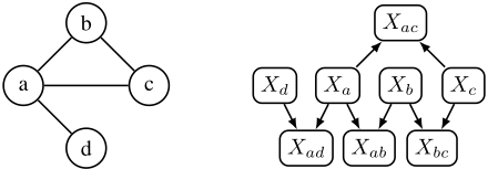
Given an instance of VERTEX COVER, construct a Bayesian network as follows. For each node v in V , add a variable Xv with P(Xv = 1) = 3/4. For each edge e = (u, v) in E, add a node Xe whose parents are Xu and Xv, and specify Xe ⇔ Xu ∧Xv. Intuitively, the nodes Xv = 0 if node v is in a vertex cover and Xv = 1 otherwise, whereas Xe = 0 if the edge e is covered by some of its endpoints, otherwise Xe = 1. The Bayesian network on the right in Figure 2 is obtained from a VERTEX COVER problem with the graph on the left. Consider an assignment v to the node variables {Xv : v ∈ V }, and denote by v(Xv) the assignment of variable Xv, v ∈ V . Let C(v) = {v : v(Xv) = 0} be the node set represented by v. By construction, if C(v) is not a vertex cover (i.e., if there is Xe such that both its parents are assigned the value one in v), then P(V = v, {Xe = 0, e ∈ E}) = 0, since P(Xe = 0|Xu = v(Xu), Xv = v(Xv)) = 0 for some e = (u, v) ∈ E. On the other hand, if C(v) is a vertex cover then P(V = v, {Xe = 0, e ∈ E}) = ∏v∈C(v) (1 - P(Xv = 1)) ∏v̸∈C(v) P(Xv = 1) = 3n-|C|/4n , where n = |V |. Hence, there is an edge cover C of size |C| ≤ k if and only if maxv P(V = v, {Xe = 0, e ∈ E}) ≥ 3n-k /4n .

Theorem 2. MPE+d (Prop(∧, (¬)) and MPE0d (Prop(∨)) are in P.

Proof. For solving MPE+d (Prop(∧, (¬)), propagate the evidence by making all ancestors of evidence nodes take on value one (true), which is the only configuration assigning positive probability. Now, for both MPE+d (Prop(∧, (¬)) and MPE0d (Prop(∨)), the procedure is as follows. Assign values of the remaining root nodes as to maximize their marginal probability independently (i.e., for every non-determined root node X select X = 1 if and only if P(X = 1) ≥ 1/2). Assign the remaining internal nodes the single value which makes their probability non-zero. This can be done in polynomial time and achieves the maximum probability.

Theorem 3. MPE+d (Prop(∨)) is NP-complete.

Proof. The proof is similar to the proof of Theorem 1. Given an instance of VERTEX COVER with graph G = (V, E) and integer k, construct a Bayesian network containing nodes Xv, v ∈ V , associated with the probabilistic assessment P(Xv = 1) = 1/4 and nodes Xe, e = (u, v) ∈ E, associated with the logical equivalence Xe ⇔ Xu ∨ Xv. Let C(v) = {v : v(Xv) = 1. Then P(V = v, {Xe = 1, e ∈ E}) = ∏v∈C(v) P(Xv = 1) ∏v̸∈C(v) (1 - P(Xv = 1)) = 3n-|C|/4n ≥ 3n-k /4n if and only if C(v) is s vertex cover of cardinality at most k.

Theorem 4. MPE+d (Prop(⊕)) is in P.

Proof. The operation ⊕ is supermodular, hence the logarithm of the joint probability is also supermodular and the MPE problem can be solved efficiently [Nemhauser et al., 1978].

3.3 MAP

Theorem 5. MAP+d (Prop(∨)) is NP PP -complete.

Proof. Consider the following NP PP -complete problem, known as EMAJ(3)SAT [Littman et al., 1998; Park and Darwiche, 2004]:

Input: A 3-CNF formula ψ(X1, . . . ,Xn) and an integer k.

Question: Is there an assignment to X1, . . . ,Xk such that the majority (that is, at least 1/2 · 2n-k ) of the assignments to Xk+1, . . . ,Xn satisfies ψ?

To prove the desired result, we first prove NP PP -hardness of an intermediate problem, which is a variant of EMAJ(3)SAT. Given a formula in CNF over X1, . . . ,Xk, we say that an assignment respects the 1-in-3 rule if at most one literal in each a clause takes on true (and to satisfy the formula, at least one needs to be true). The E(1-in-3)SAT problem is:

Input: Given a 3-CNF formula φ(X1, . . . ,Xn) with m clauses and integer k.

Question: Is there an assignment to X1, . . . ,Xk such that at least 1/21+m of the assignments to Xk+1, . . . ,Xn respect the 1-in-3 rule and satisfies φ?

We will derive a parsimonious reduction from EMAJ(3)SAT to E(1-in-3)SAT. Let m′ be the number of clauses of a EMAJ(3)SAT instance with formula ψ over n variables, and denote by R(l1, l2, l3) the relation that is true if and only if exactly one of its literals l1, l2, l3 is true. Clauses of E(1in-3)SAT will be represented by such relation as follows: each clause li,1 ∨ li,2 ∨ li,3 of EMAJ(3)SAT can be written as the set R(¬li,1, ai, bi) ∧ R(li,2, bi, ci) ∧ R(¬li,3, ci, di) ∧ R(ai, ci, ei) ∧ R(ai, ci, ei) of clauses of the E(1-in-3)SAT problem, where ai, bi, ci, di, ei are new Boolean variables only appearing in these relations. The number of satisfying assignments to the latter expression equals the number of satisfying assignments to li,1∨li,2∨li,3. Consider the formula φ obtained by replacing each of the m′ clauses in ψ by such corresponding expression. The E(1-in-3)SAT problem is that of deciding whether there is an assignment toX1, . . . ,Xk such that at least 1/21+m of the 2m+n-k assignments to Xk+1, . . . ,Xn and to (Ai,Bi,Ci,Di,Ei)i=1,...,m′ (where m= 5m′ ) respect the 1-in-3 rule and satisfy φ. Since there is a one-to-one correspondence between satisfying solutions of both problems, and the E(1-in-3)SAT instance contains 5m′ more variables than the EMAJ(3)SAT instance such that 1/21+m = 1/2·2n-k 25m′+n-k , where the numerator is 1/2 of the assignments of the EMAJ(3)SAT instance and the denominator is the number of assignments of the E(1-in-3)SAT instance, we obtain that E(1-in-3)SAT is NP PP -hard.

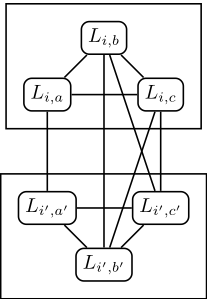
We now prove the desired result (i.e., hardness of MAP+d (Prop(∨))) by a reduction from E(1-in-3)SAT. Let R(li,1, li,2, li,3) represent the clause i of the E(1-in-3)SAT formula φ (i ∈ {1, . . . ,m}) and let Xj ∈ {0, 1} be the j-th Boolean variable (j ∈ {1, . . . , n}). Let Xi,r be the variable appearing in the literal li,r. For each literal li,r appearing in φ, create a root node Li,r in the network (there might be multiple root nodes corresponding to the same Boolean variable; nodes will be denoted with uppercase L and literals of the formula with lowercase l). Define P(Li,r = 1) = ε and interpret the state 0 of the node Li,r to mean that the literal li,r is set to true as for the satisfiability of the formula φ. Now, for each pair of literals (li,r, li′ ,r′) such that Xi,r = Xi′ ,r′ and li,r = ¬li′ ,r′ , include a disjunction evidence node Ei,r,i′ ,r′ with positive observation on it (that is, observe state 1). This will eventually force the values of nodes Li,r and Li′ ,r′ not to be 0 (that is, true) at the same time, as desired. We use the notation Ei,r,i′ ,r′ to indicate the logical relation implicitly, that is, Ei,r,i′ ,r′ ⇔ Li,r ∨Li′ ,r′ . Now, for each clause i, build three disjunction evidence nodes Ei,1,i,2, Ei,1,i,3, Ei,2,i,3 and set the observation to be positive on them (state 1), so no two literal nodes in a clause can be 0 at the same time (this implies each clause will have at most one literal node with state 0, enforcing the 1-in-3 rule). Examples of this "clause gadget" can be seen inside the dashed rectangles in Figure 3.

With the transformation so far, we already know that every configuration for the root nodes that does not respect the 1-in-3 rule will lead to a joint probability of zero, so we conclude that there are at most 4m configurations with non-zero probability. We can also state that an arbitrary assignment x1, . . . , xn of the Boolean variables in the E(1-in-3)SAT problem satisfying φ and respecting the 1-in-3 rule will have a corresponding configuration for all root nodes in the network by setting the literal nodes according to the literals in the formula (and by using the satisfying assignment x1, . . . , xn). Such configuration of the root nodes will have probability α = (1 - ε)m · ε2m, because exactly one literal node per clause will be set to state 0 and two nodes to state 1. Recall that we interpret the state zero 0 of a literal node in the network as defining such literal as true (thus state 1 means to assign false to the literal). Now take a configuration of the root nodes in the network corresponding to a situation where at least one clause of φ is not satisfied, that is, where all literal nodes corresponding to a clause in φ are set to state 1. This configuration will have probability at most β = (1 - ε)m-1 · ε2m+1 .

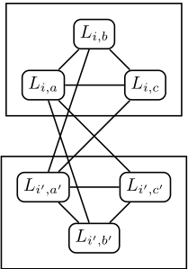
The issue still to be addressed in this reduction is that there are many configurations for the root nodes that are logically incompatible but may reach probability α (for example, take two clauses R(l1,x, l1,y, l1,z) and R(l2,t, l2,w, l2,z) where X1,z = X2,z and l1,z = l2,z and set the nodes L1,x = 0 and L2,z = 0, while leaving L1,y = L1,z = L2,t = L2,w = 1; this is possible according to the transformation but does not correspond to a valid assignment of the original Boolean variables because L1,z should be equal to L2,z). To avoid such scenarios (as well as scenarios with other incompatible literal nodes about the same Boolean variable), we define additional disjunction nodes in the network. For each two clauses i and i′ sharing a variable Xi,a = Xi′ ,a′ such that li,a = ¬li′ ,a′ , create disjunction evidence nodes Ei,b,i′ ,b′ , Ei,b,i′ ,c′ , Ei,c,i′ ,b′ , Ei,c,i′ ,c′ which will guarantee that if Li,b = 0 or Li,c = 0 then Li′ ,a′ = 0 and Li,a = 1 in any satisfying assignment, and analogously we have that if Li′ ,b′ = 0 or Li′ ,c′ = 0 then Li,a = 0 and Li′ ,a′ = 1 in any satisfying assignment (we do not care about configurations related to non-satisfying assignments because they have very low probability, as we will see). This is illustrated on the left side of Figure 3. For each two clauses i and i′ sharing a variable Xj = Xi,a = Xi′ ,a′ appearing in the literals li,a = li′ ,a′ , include disjunction evidence nodes Ei,a,i′ ,b′ , Ei,a,i′ ,c′ , Ei,b,i′ ,a′ , Ei,c,i′ ,a′ , which will force literals Li,a and Li′ ,a′ to be compatible in both clauses in any satisfying assignment. This is illustrated on the right side of Figure 3. With such additional constraints, configurations of the root nodes that are incompatible get zero probability.

Because at most 4m configurations can have non-zero probability (in fact, because of the compatibility constraints we have included, possibly less than 4m root node configurations can have non-zero probability), the sum of all configurations that correspond to assignments not satisfying φ is at most 4m · β. By choosing a value of ε such that 4m · β = 4m · (1 - ε)m-1 · ε2m+1 < 2-m-1α = 2-m-1 (1 - ε)m · ε2m ⇐⇒ 23m+1 < 1ε - 1 ⇐⇒ ε < 1 23m+1+1 , we can tell exactly the number of satisfying assignments of φ as a multiple of α with a error less than 2-m-1 (all non satisfying assignments summed together will not change this value enough to reach the next multiple of 2-m-1α).

Now we choose as MAP variables all of those related to literals that contain variables X1, . . . ,Xk, that is, M = {Li,a | Xi,a ∈ {X1, . . . ,Xk}, i ∈ {1, . . . ,m}}. We pose the query to the MAP problem of whether there is a configuration m for the MAP variables such that P(m) ≥ 2-m-1+n-k α, which happens if and only if given Boolean variables X1, . . . , Xk fixed according to m (which represents a valid assignment otherwise P(m) = 0), at least 2-m-1 assignments to Xk+1, . . . ,Xn, satisfy φ. The answer is affirmative if and only if E(1-in-3)SAT answer is affirmative, hence MAP+d (Prop(∨)) is NP PP -hard (pertinence in NP PP is immediate as it is contained in the class of MAPd problems).

Proof. MAP+d (Prop(∨)), which is NP PP -complete by Theorem 5, can be reduced to MAPd(Prop(∧)) by inverting the meaning of all nodes' states and by applying de Morgan's law to the network. Hence, all disjunctions become conjunctions and evidence nodes become all negated, hence MAPd(Prop(∧)) is NP PP -hard. As MAPd is itself a problem in NP PP , completeness follows trivially.

Theorem 7. MAP0d (Prop(∧)) and MAP0d (Prop(∨)) are PPhard.

Proof. We reduce MAJ-2MONSAT to MAP0d (Prop(∧)), which is PP-complete [Roth, 1996]:

Input: A 2-CNF formula φ(X1, . . . ,Xn) with m clauses where all literals are positive. Question: Does the majority of the assignments to X1, . . . ,Xn satisfy φ?

The transformation is as follows. For each Boolean variable Xi, build a root node such that P(Xi = 1) = 1/2. For each clause Cj with literals xi and xk (note that literals are always positive), build a conjunction node Ej with parents Xi and Xk, that is, Ej ⇔Xi ∧Xk. Now set all non-root nodes to be MAP nodes, that is, M= {E1, . . . ,Em}.

Suppose that variables in M are chosen to be m where at least one of them is set to state 1. This implies that both parents of this conjunction node must be set to state 1 too, and thus the joint probability P(m) ≤ 12 · 12 = 1 4 (as there are two root nodes with their states fixed to 1). So any MAP configuration m where not all nodes are set to state 0 will have probability inferior to 14 < 12 . On the other hand, take the MAP configuration m = 0 (vector equality). In this case, by construction, P(m) is exactly the number of satisfying assignments of φ: just interpret each configuration of the root nodes such that Xi = 0 means that the Boolean variable Xi is set to true, while node Xi = 1 means false. Because the MAP nodes are set to 0, at least one of its parents need to be set to state 0, which means that the configuration satisfies the formula φ. As the MAP value is computed as a sum over all possible satisfying assignments, the obtained probability is exactly the percentage of satisfying assignments of φ. Hence it is enough to check whether exists mwith P(m) > 12 . There is such a MAP configuration (which can only happen when all MAP nodes are set to state 0) if and only if the majority of the assignments satisfies φ. In order to prove the result for MAP0d (Prop(∨)), we just use the very same reasoning with ∨ in E nodes (MAP variables will be set to 1).

4 Going relational

In our quest for increased expressivity, we can imagine moving from random variables to parameterized random variables; that is, instead of just considering e.g. proposition Rich representing whether a particular individual is rich, we might consider e.g. relation Rich(x) with x ranging over a domain of individuals, and expressing the wealth condition of each individual. The idea is that we now have parameterized random variables [Poole, 2003], and our models are templates that get instantiated by specific sets of individuals. This allows us to investigate the complexity of networks where many nodes share the same conditional probabilities. There are indeed many such relational extensions of Bayesian networks [Jaeger, 1997; Getoor et al., 2007]. Suppose that we allow each node of our networks to be associated with a relation; given a domain, we can produce all possible groundings, and build a grounded Bayesian network by connecting groundings if their corresponding relations are connected. In this paper a domain is always a finite set, so we always produce a finite Bayesian network through grounding.

The models discussed in the previous paragraph are essentially identical to relational Bayesian networks [Jaeger, 1997], in that each node is associated with a relation, and the semantics is given by grounding into Bayesian networks. The reader can find more details about the specific features of relational Bayesian networks, and their semantics, in the literature [Jaeger, 1997]. Our only change with respect to Jaeger's original relational Bayesian networks is that we adopt again Cozman and Mauá's scheme for probability specification [Cozman and Mauá, 2015]. That is, we let each root node be associated with a probability P(r) = α, where α is a rational number in [0, 1], and each non-root node be associated with a logical equivalence r(x1, . . . , xk) ⇔ φ(x1, . . . , xk), where φ(x1, . . . , xk) is a well-formed formula in some fragment of first-order logic, with the restriction that all and only logical variables associated with r are free variables in φ. See Figure 4 for an example.

Suppose we have as input a directed acyclic graph and associated probabilities and equivalences, plus a domain (a finite list of individuals), and evidence (a conjunction of assessments for groundings). By MPE we now mean the same MPE problem as before, but applied to the grounded network, with the given evidence. And similarly for the MAP problem.

However, when we focus on relational languages we can consider additional questions. For instance, in practice it may be that the size of the relational model is small, whereas the size of the evidence, or the size of the domain, is large. So we may ask: what is the complexity of MPE when the relational model is fixed, but the evidence or domain grow? We denote by DMPE the MPE problem where the size of the relational model is bounded (and assumed constant), and only evidence and domain size may change. This sort of analysis concentrates on the so-called data complexity [Cozman and Mauá, 2015].

We start with a very simple relational language [Cozman and Mauá, 2015], obtained by restricting the popular description logic DL-Lite [Calvanese et al., 2005]. Denote by DLDiet the language consisting of the set of formulas recursively defined so that any unary relation is a formula, ¬r(x) is a formula for any unary relation r, φ∧ϕ is a formula when both φ and ϕ are formulas, and ∃y r(x, y) is a formula for a binary relation r. Note that because this language contains Prop(∧), it follows that MPEd(DLDiet) is NP-complete. However, by fixing the size of the relation model, we obtain:

Theorem 8. DMPEd(DLDiet) is in P.

Proof. The proof is rather similar to the proof of polynomialtime inference by Cozman and Mauá [Cozman and Mauá, 2015]. By construction the grounded Bayesian network consists of disconnected slices, whose variables can be selected independently. Each slice can be solved by brute force conditional on the values of the existential relations; this takes time exponential in the size of the relational network that is considered bounded (hence constant time). For each assignment of values to existential relations, the values of the binary relations can be decided greedily by inspecting the marginal probability (e.g., if the existential is set to true and the probability of the corresponding relation is less than 1/2, assign an arbitrary parent relation to true and the remaining to false). The whole process takes polynomial time.

Consider now the language EL [Cozman and Mauá, 2015], inspired by the homonymous popular description logic [Baader, 2003] as defined as follows. Any unary relation is a formula in EL, φ ∧ ϕ is a formula when both φ and ϕ are formulas, and ∃y r(x, y) ∧ s(y) is a formula when r is a binary relation and s is a unary relation. For this language, a fixed bound on the size of the relational model does not reduce complexity.

Theorem 9. DMPEd(EL) is NP-complete.

Proof. Pertinence can be shown by solving the MPE in the grounded network, an MPE problem. To show hardness, consider a VERTEX COVER problem in a graph with nodes V = {v1, . . . , vn} and edges E = {e1, . . . , em} given by its incidence matrix C: C is an n-by-m matrix such that Aij = 1 if node i is incident upon edge j and zero otherwise. Note that ∑i Aij = 2 for any j. Obtain a square matrix A′ by augmenting A with zeros (i.e., if n > m add n - m zero-filled columns; if n < m add m - n zero-filled rows). Construct the relational Bayesian network specified by P(r(x, y)) = 1/2, P(s(y)) = 1/4, t(x) ⇔ ∃y r(x, y) ∧ s(y). Let N = max{n, m}, D = {1, . . . , N}. A grounding r(j, i) represents the incidence of node vi upon an edge ej . A grounding s(i) indicates whether node vi is selected in an vertex cover, while a grounding t(j) indicates whether edge ej is covered by the vertex cover. Set E = {r(i, j) = 1 : A′ij = 1}∪{r(i, j) = 0 : A′ij = 0}∪{t(j) : ∑i A′ij /2 = 1}. Hence, the evidence ensures that t(j) = 1 if and only if s(i1) = 1 or s(i2) = 1, where vi1 and vi2 are the nodes incident upon ej with j ≤ m; for j > m any assignment to s(i) satisfies the evidence t(j) = 0. The joint probability of the Bayesian network is P(s(1), . . . , s(N),E) = ∏(vi1 ,vi2 )∈E I(s(i1) ∨ s(i2)) ∏Ni=1 P(s(i)) , where I is the indicator function which returns one if its argument evaluates to true and zero otherwise. Consider an assignment s1, . . . , sN to s(1), . . . , s(N) and let C = {vi : i ≤ n, si = 1}. If C is a vertex cover then P(s(1) = s1, . . . , s(N) = sN, E) = 3N-|C|/4N ; if C is not an vertex cover then P(s(1) = s1, . . . , s(N) = sN, E) = 0. Hence maxs1,...,sN P(s(1) = s1, . . . , s(N) = sN,E) ≥ 3N-k /4N if and only if there is a vertex cover of cardinality at most k.

The proof above makes use of negated evidence on binary relations; the complexity of the problem with positive evidence (that is, DMPE+d (EL)) remains open.

5 Conclusion

In this paper we have presented complexity results for MPE and MAP problems in Bayesian networks, as parameterized by the language in which probabilities are specified. Complexity results for these problems have focused on graph topology, but it has been long known that restrictions on parameter specification lead to distinct computational behavior. Our analysis offers an initial formalization of this perception. Overall we find that disjunction is the key source of computational intractability; as long as disjunction can be represented, complexity jumps considerably.

There are many possible extensions of this work. We only barely touched relational models; there are many languages that deserve attention. Issues such as separating the effect of data size and domain size from network size are important and should also be examined.

Acknowledgments

The first author was partially supported by the São Paulo Research Foundation (FAPESP) through the grant 2013/231974. The third author was partially supported by CNPq.