Bimodal Switching for Online Planning in Multiagent Settings

1 Introduction

Online planning involves deliberating on optimal actions to perform in a limited amount of time given beliefs that evolve as the agent acts and observes. The limited-time aspect puts an emphasis on reduced planning time, which is achieved by trading off optimality and relying on approximations. Attention to online planning has predominantly focused on singleagent settings [Ross et al., 2008] albeit isolated approaches for cooperative problems do exist [Wu et al., 2011].

We attend to planning in the presence of an interacting agent, which complicates the process. In this space, the finitely-nested interactive partially observable Markov decision process (I-POMDP) [Gmytrasiewicz and Doshi, 2005; Doshi, 2012] is a recognized approach for performing the deliberations by modeling the other agent. Approaches such as the interactive particle filtering [Doshi and Gmytrasiewicz, 2009] offer a way to plan online given a belief. However, this is time consuming and does not scale well.

Within the I-POMDP framework, an agent simultaneously updates its beliefs over both the physical state and the models of other agent based on its actions and observations. The distribution over the models is updated based on the predicted action, whose effect on the state is observed by the agent. These observations become more informative when the agent's belief over the physical state has reduced uncertainty (entropy). For example, in the context of the wellknown multiagent tiger problem [Gmytrasiewicz and Doshi, 2005], let the agent strongly believe that the tiger is on the left but on listening hear a growl from the right. If the observation is reliable with a high probability, the agent infers that the other agent likely opened the door causing the tiger to change its location.

∗We acknowledge support from NSF CAREER grant, #IIS0845036.

We present a novel two-stage approach that focuses first on online planning as if the agent is alone, in order to reduce uncertainty in its belief over the physical state. In this mode, the agent is modeled as a POMDP and utilizes a fast POMDP-based planning technique, SARSOP [Kurniawati et al., 2008], that takes orders of magnitude less time to execute as compared to the I-POMDP solver. Subsequently, the agent switches to the I-POMDP model combining its updated belief over the state and the initial belief over the models. It now performs online planning using interactive particle filtering.

A key question is when should the agent switch from the POMDP to the I-POMDP mode? In order to answer this, the agent at every step computes lower and upper bounds on the optimal decision at that step. The agent switches to the latter mode when the fractional difference between the lower and upper bounds at any step become less than a parameter, ϵ. Because of the convexity property of the lower-bound value function, the difference between the two typically reduces as beliefs become less uncertain. Nevertheless, the bounds may not converge, and very small ϵ values may not cause a switch.

We estimate the error that this approach entails. The computational savings result because during the initial steps of online planning, a fast and scalable single-agent approach is utilized. We illustrate this approach on the multiagent tiger problem and show that the total time elapsed over several steps is significantly less compared to using an I-POMDP model only at the expense of reduced cumulative reward.

2 Overview of Finitely-Nested I-POMDPs

A finitely-nested I-POMDP [Gmytrasiewicz and Doshi, 2005] for an agent i with strategy level, l, interacting with another agent j is defined using the tuple:

• ISi,l denotes the set of interactive states at strategy level, l, defined as, ISi,l = S ×Mj,l-1, where S is the set of physical states, and Mj,l-1 is the set of models ascribed to the other agent.
• A = Ai ×Aj is the set of joint actions of all agents.

The remaining parameters - Ti (transition function), Ωi and Oi (observation space and function respectively), Ri (reward function), and OCi (optimality criterion) - are defined analogously to POMDPs with the generalization that the functions are conditioned on the joint actions, and the states are the physical states only. We focus on optimizing the summation of the discounted reward over a finite number of remaining steps, called the horizon.

Agent i's 0-th level belief is a probability distribution over the physical states only, and the 0-th level models, Mj,0, consist of the set of computable intentional models of level 0, Θj,0, and the subintentional models, SMj. An intentional model, θj,0 = 〈bj,0, ˆ θj〉, where bj,0 is j's level 0 belief, bj,0 ∈ △(S) - △(S) is the set of all distributions over S - and ˆ θj = 〈A, Tj,Ωj,Oj,Rj,OCj〉, is j's frame. Here, j is assumed to be Bayes-rational. 0-th level intentional models are POMDPs. An agent's level 1 beliefs are probability distributions over the physical states and level 0 models of the other. First-level models include level 1 intentional models and level 0 models of the agent, and so on up to level l.

We limit our attention to intentional models only, and simplify the interactive state space to include intentional models of the other agent that are of level one less than that of the modeling agent. We assume that the frame of agent j is known and remains fixed; it need not be the same as that of i.

An agent's belief over its interactive states, bi,l, fully summarizes the agent's observation history. We may factor the agent's belief as: bi,l(is) = bi,l(s) bi,l(θj,l-1|s). Beliefs are updated after the agent's action and observation using Bayes rule. First, as the state of the physical environment depends on the actions performed by both agents, the prediction of how it changes has to be made based on the probabilities of various actions of the other agent. Probabilities of other's actions are obtained by solving its models. Second, changes in the models of the other agent have to be included in the update. The changes reflect the other's observations and, when modeled intentionally, the update of other agent's beliefs.

Given the generalized belief update, solution to an IPOMDPi,l is a policy, analogous to that in a POMDP. Gmytrasiewicz and Doshi (2005) provide additional details on IPOMDPs, and the Bellman operator for backup, H.

One approach for online planning in settings formalized by I-POMDPi,l involves sampling the interactive state space and projecting the samples, called particles, across time in order to simulate the belief update. The interactive particle filter (I-PF) [Doshi and Gmytrasiewicz, 2009] propagates, weights and resamples a nested set of particles of level l. A reachability tree is generated where the sampled representations of beliefs at the nodes are obtained by running the I-PF. Value iteration using sample sets on the reachability tree is performed to obtain the approximately-optimal action at the given belief.

3 Bimodal Online Planning

Let b0i,l be agent i's initial belief over the interactive state space. Agent i initially views the problem as a single-agent POMDP and its belief is the distribution over the physical states only, b0i,l (s). Conditional beliefs over the models given the state, b0i,l (·|s), are held fixed. Subsequently, the agent switches to updating the conditionals as well after some steps.

We show that in problems where direct (including noisy) observations about the other agent's actions are not available and its actions are inferred by sensing the next state, perhaps noisily, knowing the current state provides greater information about the true model of the other agent.

Definition 1 (Unobservable actions). Actions of agent j are directly unobservable to agent i iff observations of i are conditionally independent of j's action, Oi(s, ai, aj, oi) = Oi(s, ai, oi); ∀ aj ∈ Aj, oi ∈ Ωi, ai ∈ Ai, s ∈ S.

Let Pr( ˙ θt+1 j,l-1 |ot+1 i , ati , bti,l ) be i's probability of the true model of the other agent, ˙ θt+1 j,l-1 , on observing, ot+1 i , and performing action, ati , given belief, bti,l . We may write it as,

Notice that the term on the right is agent i's updated belief over a state and true model of j, which is obtained using the I-POMDP belief update. Under Def. 1 applied to both agents,

(1)

where τ is an indicator function that is 1 when model, θtj,l-1 , updates to ˙ θt+1 j,l-1 on performing action, atj , and receiving observation, ot+1 j ; otherwise 0. Equation 1 shows that i's belief over j's true model at t + 1 is influenced by j's predicted actions from its models, the observations that j may likely receive and agent i's transition and observation functions.

Let agents i and j perform actions, ati and atj respectively, due to which the state transitions from st to st+1 . As j's actions are unobservable, state transitions allow valuable inference of j's actions.

Definition 2 (Maximally informative transition). The above state transition is maximally informative about j's action iff Ti(st , ati , atj , st+1 ) ≥ Ti(¯ st , ati , atj , st+1 ) for any other state, ¯ st , and T(st , ati , atj , st+1 ) > T(st , ati , ¯atj , st+1 ) for all other actions, ¯atj , of j.

Consider domains where the other agent's actions are unobservable (Def. 1). In such settings, observations are more informative about the other agent's models if the uncertainty over the physical state is mitigated. In order to show this, let the transition that occurs from the current state, ˙st , due to joint actions be maximally informative (Def. 2). Let j's performed action solely lead to its true model. Agent i then receives the observation, ot+1 i , that is most likely. Then, the following proposition holds:

Proposition 1. If bt,1 i,l is a belief which assigns probability 1 on the current state, ˙st , then, Pr( ˙ θt+1 j,l-1 |ot+1 i , ati , bt,1 i,l ) ≥ Pr( ˙ θt+1 j,l-1 |ot+1 i , ati , bt,2 i,l ), for any other belief, bt,2 i,l , under the assumption that the conditional distributions over the models of j in both beliefs are identical and do not change with state.

Proof. For convenience, we may rewrite Eq. 1 as,

where X(st , ati , ot+1 i , ˙ θt+1 j,l-1 ) denotes the remaining terms of Eq. 1 as a function of st , ati , ot+1 i , and ˙ θt+1 j,l-1 . Under the assumption that i's conditional distribution over the models is identical for any state, if the current state is ˙st , then X( ˙st , ati , ot+1 i , ˙ θt+1 j,l-1 ) is greater than X (¯ st , ati , ot+1 i , ˙ θt+1 j,l-1 ) for any other state, ¯ st . This is because, ∑ st+1 Ti(¯ st , ati , atj , st+1 ) Oi(st+1 , ati , ot+1 i ) ≤ ∑ st+1 Ti( ˙st , ati , atj , st+1 ) Oi(st+1 , ati , ot+1 i ), as any transition to a possible next state, st+1 , is maximally informative about j's action given i's action, from the current state, ˙st . While some other action of j could result in a next state, st+1 , from some ¯ st , it does not lead to the true model of j as per τ . As bt,1 i,l puts a probability 1 on ˙st , it follows that X( ˙st , ati , ot+1 i , ˙ θt+1 j,l-1 ) is greater than ∑st bt,2 i,l (st ) X(st , ati , ot+1 i , ˙ θt+1 j,l-1 ), for any other belief, bt,2 i,l , which differs from bt,1 i,l in its distribution over the physical states only.

While we sought to reduce some of the possibilities due to uncertainty, Proposition 1 formalizes the intuition that in domains where behavioral information about the other agent must be inferred by sensing the dynamic state, received observations (that are not noise) tend to be more informative about the other's model when the uncertainty over the current physical state is as less as possible.

If agent i's conditional belief over models is decoupled from its belief over the physical state, the proposition becomes useful as the beliefs, bt,2 i,l and bt,1 i,l , could be those that are in the sequence of beliefs that i may have as it acts and observes. Consequently, in problems where j's actions are unobservable, it motivates that we update the distributions over the models as late as possible in the game. Of course, the trade off is that the conditional distributions over models are held fixed for a longer time affecting early predictions.

3.1 POMDPmodel with noise

Our formulation of the POMDP model [Kaelbling et al., 1998] for agent i, POMDPi, uses as its state space the set of physical states, S, in the I-POMDPi,l. The action and observation spaces are identical to those in I-POMDPi,l. The transition, observation, and reward functions are marginals of those in I-POMDPi,l, obtained by summing out j's actions from the functions. The optimality criterion remains a sum of discounted rewards over the finite horizon.

In order to sum out j's actions from the functions, we begin by mapping j's model space to a set of nodes, Nj,l-1. Each node in this set corresponds to a distribution over j's actions. If j is at level 0, we obtain these nodes by performing bounded policy iteration (BPI) [Poupart and Boutilier, 2003] on the level 0 POMDP, which is a technique for obtaining a controller of fixed size. Our BPI begins with a single node that corresponds to a random action followed by one step of full backup. Subsequently, the controller is improved using BPI until convergence. Let Nj,l-1 be the set of nodes of this converged controller. Associated with each node is also a value vector that gives the expected reward of performing the action(s) corresponding to the node from each state, and then following the remaining controller until the values converge.

Nodes in Nj,l-1 partition the continuous model space: For a belief, bj,0, in each model, compute the inner product between the belief and the value vector for each node. Then, map the model to the node with the largest value breaking ties randomly. Note that multiple models may be mapped to a single node. For j's models at a level, l - 1, greater than 0, we may perform interactive BPI [Sonu and Doshi, 2012] resulting in a (nested) controller of level l - 1. A benefit of this approach of mapping models to nodes is that the countably infinite model space is reduced to a finite set of nodes, Nj,l-1. We may obtain the distribution over j's actions for summing out as:

where Pr(aj|nj,l-1) is the probability assigned to action, aj, by the node, nj,l-1, and b0i,l (nj,l-1|s) is the conditional probability mass in i's initial belief over models that get transferred to nj,l-1 due to the mapping: b0i,l (nj,l-1|s) =

Equation 2 provides the distribution over the other agent's actions used for formulating the marginal functions. This distribution is static and the resulting POMDPi models the other agent as noise in the environment. Solution of this POMDP is obtained by using SARSOP [Kurniawati et al., 2008], which is a fast and scalable POMDP solution technique that produces a policy graph.

Next, we show that the expected reward from our formulation of POMDPi is a lower bound to the expected reward from I-POMDPi,l in which the model space, Θj,l-1 has been substituted with the space, Fj,l-1. Here, fj,l-1 ∈ Fj,l-1 is, fj,l-1 = 〈nj,l-1, ˆ fj,l-1, ˆ θj〉, where nj,l-1 is a node in the set of nodes in j's level l - 1 controller, nj,l-1 ∈ Nj,l-1; ˆ fj,l-1 includes the set of edge labels, distributions of actions for each node and the edge transition function of the controller; and ˆ θj is j's fixed frame. In other words, treating the other agent as noise is less valuable than correctly modeling it.

In order to compare between the two value functions, we obtain the value of i's marginal belief over the physical state in the I-POMDPi,l as: V (bi,l(s)) = max ˆα ∑ s∈S bi,l(s) ˆα(s).

Here,

where b0i,l (nj,l-1|s) is the initial conditional belief over nodes as defined previously, and α(s, nj,l-1) is an alpha vector that composes the value function for I-POMDPi,l.

Proposition 2 (Lower bound). Let V denote the value function of I-POMDPi,l. Let H and H be the backup operators for POMDPi and I-POMDPi,l, respectively. Then, it holds that HV ≥ HV .

Proof. Let bi,l(s) be a belief over the physical states, and bi,l(s, nj,l-1) = bi,l(s) b0i,l (nj,l-1|s), where b0i,l (nj,l-1|s) is the initial conditional distribution.

We begin by showing that for horizon 1, for any bi,l(s), value of this belief given by POMDPi is the same as the value of the belief, bi,l(s, nj,l-1), shown previously:

where ˆRi(s, ai) is agent i's reward function in POMDPi. Introducing aj gives,

Next, we move to the case where the horizon is 2, and apply the I-POMDPi,l backup operator to the value function, V :

where k is the index of the alpha vector that provides the maximal value at the updated belief, b′i,l . We may rewrite the above dynamic programming update by noting that ∑oj Oj(s′ , aj, oj) ∑ n′j,l-1 Pr(n′j,l-1 |nj,l-1, ai, oj) rep-

resents the updated belief over the models conditioned on the updated state, b′j,l-1 (n′j,l-1 |s′ ).

The above holds because αk (s′ , n′j,l-1 ) is maximal at b′i,l = b′i,l (s′ )b′i,l (n′j,l-1 |s′ ). For the belief in the above equation, b′i,l (s′ )b0i,l (n′j,l-1 |s′ ), it may continue to remain maximal if b′i,l (n′j,l-1 |s′ ) and b0i,l (n′j,l-1 |s′ ) are identical, otherwise it's suboptimal. Using Eq. 3, above equation may be rewritten.

Here, ˆR is the reward function in POMDPi as defined previously, Pr(s′ , oi|s, ai) is the joint observation and transition functions, and H is the corresponding backup operator.

As V = V , we also get, HV ≥ HV from the above proof, and furthermore, H(HV ) ≥ H(HV ). Because the IPOMDPi,l backup operator is isotonic, H(HV ) ≥ H(HV ). This implies, H(HV ) ≥H(HV ). Thus, repeatedly applying the two backup operators maintains the lower bound.

This is intuitive and demonstrates the benefit of closely tracking the other agent's dynamic models.

3.2 I-POMDPi,l with perfectly observable state

As we mentioned previously, agent i utilizes the policy graph resulting from solving POMDPi using a fast and scalable technique. The value of the action given by POMDPi for any i's belief over the physical states is guaranteed to be a lower bound to the optimal approach of using I-POMDPi,l. Eventually, the agent switches to using an online solution of I-POMDPi,l for acting. In order to facilitate the switching, an upper bound value for its belief over the physical states is additionally needed.

If an observation reveals the physical state perfectly to agent i in an I-POMDPi,l, the proposition below shows that the resulting value of bi,l is an upper bound to the general value. Notice that despite the physical state being perfectly observable, the resulting model does not collapse into an MDP because the model of the other agent continues to remain uncertain. Let V be the value function of this model, which we denote as I-POMDPSi,l . The value function is composed of possibly multiple vectors for each state, s. For each state, we obtain the maximal value of the inner product between the initial conditional belief, bi,l(nj,l-1|s), and the updated alpha vectors for that state. These values form a single alpha vector over the physical states.

Proposition 3 (Upper bound). Let H be the backup operator for the value function of I-POMDPSi,l as defined in Eq. 4. Then, it holds that HV ≤ HV , where H is the backup operator for I-POMDPi,l as defined previously.

For a horizon greater than one, we obtain,

The alpha vector, αs′ ,k′ (n′j,l-1 ), is the one in the set of vectors for the next state, s′ , that gives the largest value for the updated conditional belief over the models. Its selection from the set does not depend on the observation, oi, unlike in IPOMDPi,l. Therefore, the equation above simplifies to,

Under the isotonicity property of the I-POMDP backup operator and V ≤ V , we obtain, H(HV ) ≤ H(HV ). Similarly, H(HV ) ≤ H(HV ). We may reapply the above proof and assert that, H(HV ) ≤ H(HV ). This implies that, H(HV ) ≤ H(HV ), which means that the upper bound is maintained over any number of applications of the two backup operators to their respective value functions.

3.3 Bimodal switching

Let the difference between the upper and lower bound values for a belief, bi,l, over the physical states be, Diff = V i(bi,l) - V i (bi,l). Let Rmin and Rmax be the smallest and highest rewards in agent i's reward function, Ri. Subsequently, Rmin 1-γH 1-γ and Rmax 1-γH 1-γ are the minimum and maximum rewards that agent i could obtain over a finite horizon of H with a discount factor of γ. These may be easily calculated from the model definition.

Because of the piecewise linear and convexity property of the value function of POMDPi, and the relatively flat value function of I-POMDPSi,l , we expect Diff to reduce as the uncertainty in agent i's belief over the state space reduces and the belief approaches the edges of the belief simplex. Our approach switches from online planning using POMDPi to planning using I-POMDPi,l when Diff·(1-γ) (1-γH )·(Rmax-Rmin) drops to below a parameter, ϵ ∈ [0, 1]. In other words, ϵ is the fraction of the largest possible difference in value, which triggers the switch. However, not all values of ϵ may be reached. Specifically, there is no guarantee that the upper and lower bounds converge near the edges of the belief simplex. Consequently, small values of ϵ may not cause a switch.

3.4 Computational Savings and Error Bound

Instead of solving a multiagent planning problem from the start, our approach exploits single-agent planning in the early stages subsequently switching to multiagent planning on reaching a belief distribution that admits reduced error bound. Consequently, computational savings occur due to the steps when single-agent planning is performed. In order to obtain an estimate of the savings, let us suppose that we use an exact POMDP-based approach for online planning that generates a perfect reachability tree of H - 1 steps whose branching factor is (|Ai||Ωi|), from a belief. The tree contains (|Ai||Ωi|)H - 1 nodes each of which is associated with a single real number whose computation takes time O(|Ai||S|) if the node is a leaf node, otherwise it takes O(|Ai||Ωi||S|2 ). On the other hand, let us suppose that we use an exact I-POMDPi,l-based approach for the planning. The reachability tree from a belief over the interactive state space would continue to have a branching factor of (|Ai||Ωi|) and as many nodes as mentioned previously. However, calculating the value of the belief associated with each leaf node takes time O(|Ai||S||Nj,l-1||Aj|) and the time for calculating the value at a non-leaf node takes O(|Ai||S|2 |Nj,l-1||Aj|Ωi||Ωj|). The difference in computation time at each node is due to modeling the other agent, and the savings at all the nodes accumulates over the number of steps for which planning uses POMDPi, which may vary.

Our choice of SARSOP - a state of the art approach - minimizes the time taken to perform the POMDP-based planning. SARSOP generates a policy graph that is near-optimal for a given horizon from any belief, and the initial computation time is amortized over the multiple steps for which the graph is used. The I-POMDPi,l-based online planning utilizes I-PF and generates a reachability tree for a given horizon from a given belief resulting in an approximate action.

If an exact approach is utilized for online multiagent planning after the switch, error is incurred until the approach switches when ϵ is achieved. At this point, the difference between the upper and lower bounds is, ϵ· (1-γH )·(Rmax-Rmin) 1-γ , which bounds the error as well. If T steps were performed before switching, then the error is at least, T · ϵ · (1-γH )·(Rmax-Rmin) 1-γ . This also serves as a reasonable estimate of the error because our bounds are tight resulting in small ϵ values, as we illustrate next.

4 Experimental Evaluation

In Figure 1, we illustrate the lower and upper bound values for changing beliefs of agent i over the physical states for the multiagent tiger problem [Gmytrasiewicz and Doshi, 2005]. We modify this problem by removing creaks thereby making j's actions unobservable (Def. 1) and let the tiger persist with a probability of 0.75 in its original location after a door is opened. Furthermore, we mitigate the amount of noise in j's observations of the state as modeled by i to 0.05.

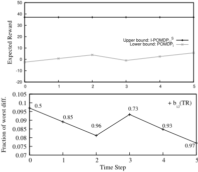
Beginning at a belief of bi,1(TR) = 0.5 indicating that the tiger is believed to be behind the right door with a probability of 0.5, the beliefs are updated as the agent listens and receives observations. We obtained j's controller using BPI, which has 5 nodes. Agent i's initial distribution over these nodes is obtained by mapping a distribution over level 0 models of j to a distrbution over the nodes. Notice that the fraction, ϵ, becomes smaller as the beliefs show less uncertainty although not monotonically. The increase from steps 2 to 3 occurs due to i opening the left door causing the uncertainty in its beliefs to increase and reducing the lower bound value.

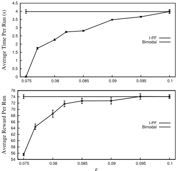
Taking an online planning horizon of H = 5, we simulated agent i's play of the tiger problem for 30 steps. We vary ϵ and show the time and cumulative reward averaged over 5 trials of 300 simulation runs each. Notice the low values of ϵ indicating that our bounds are tight. The feasible range of ϵ is [0.075,0.1], with the approach unable to reach ϵ < 0.075 and degenerating into POMDPi for all the steps, while satisfying ϵ < 0.1 at the first step itself thereby running using I-PF for all the steps. For the smallest ϵ value which causes a bimodal switch, the average time is about 50% less than I-PF albeit obtaining average reward that is significantly lower. However, as ϵ increases, POMDPi runs for less steps and both the time and rewards increase approaching that of I-PF.

5 Conclusion

We presented a new approach for online planning in multiagent settings where actions of the other agent are not directly observable and must be inferred from the state transitions. For typical initial beliefs with high uncertainty over the physical states, our approach utilizes POMDP-based planning and switches over to online multiagent planning. The mode changes when the fraction of the difference between the upper and lower bounds reduces to less than a parameter. This technique of utilizing bounds is analogous to previous approaches such as HSVI [Smith and Simmons, 2004] and SARSOP, although these compute bounds relevant to single agent settings. Our demonstration on a toy problem domain indicates that the bimodal approach is flexible and significantly saves on time while obtaining improved rewards.