
Flexibility and Decoupling in the Simple Temporal Problem
Proceedings of the Twenty-Third International Joint Conference on Artificial Intelligence. Pages 2422-2427.
© 2013 International Joint Conferences on Artificial Intelligence
Abstract
In this paper we concentrate on finding a suitable metric to determine the flexibility of a Simple Temporal Problem (STP). After reviewing some flexibility metrics that have been proposed, we conclude that these metrics fail to capture the correlation between events specified in the STP, resulting in an overestimation of the available flexibility in the system. We propose to use an intuitively more acceptable flexibility metric based upon uncorrelated time-intervals for the allowed starting times of events in an STP. This metric is shown to be computable in low-polynomial time. As a byproduct of the flexibility computation, we get a decomposition of the STN almost for free: for every possible k-partitioning of the event space, a decomposition can be computed in O(k)-time. Even more importantly, we show that contrary to popular belief, such a decomposition does not affect the flexibility of the original STP.
- [Boerkoel and Durfee, 2011] J.C. Boerkoel and E.H. Durfee. Distributed algorithms for solving the multiagent temporal decoupling problem. In Proceedings AAMAS, 2011.
- [Boerkoel and Durfee, 2012] J.C. Boerkoel and E.H. Durfee. A distributed approach to summarizing spaces of multia- gent schedules. In Proceedings AAAI, 2012.
- [Boerkoel, 2012] J.C. Boerkoel. Distributed Approaches for Solving Constraint-based Multiagent Scheduling Prob- lems. PhD thesis, University of Michigan, 2012.
- [Brambilla, 2010] A. Brambilla. Artificial Intelligence in Space Systems: Coordination Through Problem Decou- pling in Multi Agent Planning for Space Systems. Lambert Academic Publishing, 2010.
- [Dechter et al., 1991] R. Dechter, I. Meiri, and J. Pearl. Tem- poral constraint networks. Artificial Intelligence, 49:61- 95, 1991.
- [Dechter, 2003] R. Dechter. Constraint processing. Morgan Kaufmann, 2003.
- [Floyd, 1962] R.W. Floyd. Algorithm 97: Shortest path. Communications of the ACM, 5(6):345, 1962.
- [Hunsberger, 2002] L. Hunsberger. Algorithms for a tempo- ral decoupling problem in multi-agent planning. In Pro- ceedings AAAI, 2002.
- [Morris et al., 2001] Paul H. Morris, Nicola Muscettola, and Thierry Vidal. Dynamic control of plans with temporal uncertainty. In Proceedings IJCAI, pages 494-502, 2001. IJCAI
- [Planken et al., 2010] L. Planken, M. de Weerdt, and C. Wit- teveen. Optimal temporal decoupling in multiagent sys- tems. In Proceedings AAMAS, 2010.
- [Policella et al., 2007] N. Policella, A. Cesta, A. Oddi, and S.F. Smith. From precedence constraint posting to partial order schedules: A CSP approach to robust scheduling. AI Communications, 20:163-180, 2007.
References were extracted automatically from the PDF and may contain errors.
Full text extracted automatically from the PDF; figures, tables and equations may differ. The PDF is the version of record.
1 Introduction
Scheduling problems occur in many diverse application domains such as transportation, process industry, health and education. Intuitively, a scheduling problem arises if there is a set of temporal events whose (starting) times are subject to a number of temporal constraints and we have to determine these starting times such that all constraints are satisfied. Usually, we are not satisfied with determining a single schedule, i.e., an assignment σ determining for every event t an exact starting time σ(t). First, due to outside disturbances (e.g., unforeseen delays), it may not be possible to start event t at the predetermined time. Then it is essential for the scheduling agent to know how to maintain or adapt the current schedule. Since during execution there is not much time for rescheduling, the possibilities for alternative starting times should be computable in a very short time or, even better, known in advance. Therefore, instead of offering a fixed schedule as a solution, one would like to compute an interval schedule, that is, an assignment of time intervals to variables, such that for every event t one can freely choose a specific time point in its interval. Such an interval for event t indicates the flexibility we have w.r.t. starting t. The sum of such flexibilities then indicates the flexibility of the interval schedule and could be used to measure its quality in this respect.
Another reason to opt for scheduling with time intervals occurs when the scheduling problem is distributed among multiple actors who want to solve the overall scheduling problem. Typically, such agents want to schedule their part of the problem independently of the others, based on their own preferences. One method that has been applied to fairly general scheduling formalisms is known as temporal decoupling [Hunsberger, 2002]. Here the original scheduling problem is decomposed into a number of subproblems, such that any solution (i.e., schedule) to a subproblem can be merged with any solution of the other subproblems, to constitute a feasible schedule of the total problem. As has been pointed out by various authors [Hunsberger, 2002; Planken et al., 2010; Boerkoel and Durfee, 2011; Brambilla, 2010], when using existing flexibility metrics, applying temporal decoupling may affect the total flexibility of the system. The question then arises, how we could minimise this flexibility loss due to temporal decoupling. Hence, we would also like to (i) optimize the decoupling with respect to flexibility and, if necessary, (ii) investigate the loss of flexibility due to decoupling.
Our approach to addressing these problems is the following. We will concentrate on Simple Temporal Planning (STP) problems [Dechter, 2003] as the main representation mechanism for (temporal) scheduling problems. After a discussion of existing metrics to characterise the flexibility of STPs, we show that these metrics are not able to capture correlated time events, and generally overestimate the flexibility of scheduling systems. Then we introduce a new flexibility metric by using a transformation from a given STP S into a new STP S′ such that correlations between time points are resolved in S′ . By using an LP-approach to finding a simple uncorrelated interval schedule for events in S′ , we can obtain the flexibility of the original system S. We show that in case of STPs this flexibility metric can be computed in polynomial time and offers the possibility to adapt existing schedules in O(1) time. Then we deal with the problem of finding an optimal temporal decoupling for a given STP. Surprisingly, the method we use to specify the flexibility of an STP allows us to compute a decoupling for an STP that does not induce any loss of flexibility due to decoupling and can be obtained in O(k)-time (if the flexibility of the system has already been computed), where k is the number of agents involved in the decoupling.
This result shows that temporal decoupling can be computed both efficiently and without loss of flexibility.
2 Preliminaries
The Simple Temporal Problem [Dechter et al., 1991; Dechter, 2003], offers a convenient framework for analyzing temporal aspects of scheduling problems, distinguishing between a set of temporal variables and linear constraints between them.
An instance of the Simple Temporal Problem (STP) is a pair S = (T, C), where T = {t0, t1, . . . , tn} is a set of timepoint variables (events) and C is a finite set of binary constraints on T , each constraint having the form tj - ti ≤ cji, for some real number cji. Given S, we want to find a schedule for the events in T, that is a function σ : T → R≥0 , assigning a non-negative real value (time-points) to each event in T , such that all constraints in C are satisfied. If such a schedule exists, we say that the STP is consistent. Without loss of generality, in the remaining of the paper, we simply assume that an STP is consistent. 1
In order to be able to express absolute time constraints, the time-point t0, also denoted by z, is used. It represents a fixed reference point on the timeline, usually having the value 0.
Often we represent an STP S = (T,C) as a directed labeled graph where the vertices represent events in T and for every constraint tj - ti ≤ cji in C there is a directed edge (ti, tj) labeled by cji. The graph associated to an STP is called a Simple Temporal Network (STN). In this paper, we will use both representations interchangeably.
Example 1. In Figure 1 two STNs S1 and S2 are given, both representing an STP with three time events (including the time reference point z). From these graphs we can derive the specification of the associated STPs. For example, the STP associated to S1 contains a constraint t2 - t1 ≤ 5 and a constraint t1 - t2 ≤ -5, while the STP belonging to S2 contains a constraint t2 - t1 ≤ 0 and a constraint t1 - t2 ≤ 5.
The graph representation is very helpful in finding constraints implied by the set C of constraints, interpreting the weights cji on the arcs as lengths of the path from ti to tj. For example, if C contains the constraints tj - ti ≤ 10 and tk - tj ≤ 15, then there exists a path from ti via tj to tk having a length 10 + 15 = 25. This implies tk - ti = (tk - tj) + (tj - ti) ≤ 25 is an implied constraint , even though C may not have contained a constraint limiting tk-ti. Using a shortest path interpretation of the STN S = (T, C), there is an efficient method to find all tightest constraints implied by C. Basically, these tightest constraints can be found by searching for all shortest paths between the time points in T by e.g. applying Floyd and Warshalls all-pairs shortest paths algorithm [Floyd, 1962]. These tightest constraints are represented as the elements of the n × n distance matrix DS, containing for every pair of time-point variables ti and tj the length of the shortest path in the distance graph between ti and tj. If DS contains the entries DS[i, j] and DS[j, i], then -DS[j, i] ≤ tj-ti ≤ DS[i, j] are the strongest constraints implied by C w.r.t. the temporal difference between tj and ti. The first row of DS contains all entries DS[0, i] such that ti - z = ti ≤ DS[0, i], so DS[0, i] is ti's latest starting time, lst(ti). Analogously, the first column contains entries DS[j, 0] such that z - tj ≤ DS[j, 0], i.e., tj - z = tj ≥ -DS[j, 0], so -DS[j, 0] is tj's earliest starting time, est(tj). The distance matrix DS for a given STN S can be computed in O(n3 ) time [Dechter, 2003]. Hence, using the STP machinery we can find earliest and latest starting times for events in O(n3 ) time.
1 Consistency of an STP can be determined in low-order polynomial time.
The following proposition is a summary of two relevant properties that can be proven to hold for STNs and their schedules:
Proposition 1. Let S = (T,C) be an STN and DS its distance matrix. For i = 1, . . . , n, let est(ti) = DS[0, i] and lst(ti) = -DS[i, 0]. Then, for every schedule σ for S, and every t ∈ T, it holds that σ(t) ∈ [est(t), lst(t)]. Moreover, given any t ∈ T and v ∈ [est(t), lst(t)], there exists 2 a schedule σ for S such that σ(t) = v.
Since we want to solve scheduling problems using STNs, we assume that for each event t there is a finite horizon for scheduling it. That means that for each STN S = (T, C) we assume that there exists a finite constant hS such that for all t ∈ T it holds that t ≤ hS can be derived fromC. This avoids the use of unbounded time intervals (e.g. ti - tj ≤∞).
3 Flexibility of an STN
Intuitively, the flexibility of an STN refers to the amount of freedom we have in assigning times to events in T. We defined a fixed schedule σ for an STN S = (T,C) as an assignment σ : T → R≥0 satisfying all the constraints in C. Such a schedule, however, is just an arbitrary fixed assignment among a large set of possible alternative assignments also satisfying the constraints. Therefore a single fixed schedule does not offer any indication of the flexibility of the STN it has been derived from.
Using Earliest and Latest Starting Times
If we want flexibility to indicate our freedom of choice, then one option for defining the flexibility for scheduling event t is to use the difference lst(t) - est(t) = flexN(t). The total flexibility flexN(S) of S then could be defined as
Obviously, flexN(S) can be computed in O(n3 ) time. Moreover, for each individual t, flexN(t) gives an exact measure of flexibility of event t, since, by Proposition 1, for every choice of a value v ∈ [est(t), lst(t)] there exists a schedule σ for S such that σ(t) = v. However, although for every individual event, flexN(t) offers a precise measure of its flexibility, using the sum flexN(S) of these flexibilities has a serious disadvantage, due to correlations that might exist between starting times of events. To see this, consider the following example:
2 In fact it can be shown that there exists a simple backtrack-free polynomial-time algorithm to construct an arbitrary schedule σ for S.
Example 2. Consider the STNs S1 and S2 (see Figure 1) where S1 specifies the concurrent execution of k = 3 events within 5 time units, while S2 specifies the sequential execution of k = 3 consecutive events, i.e., t2 should not occur before t1, while t3 should not occur before t2 and all should occur within 5 time units.
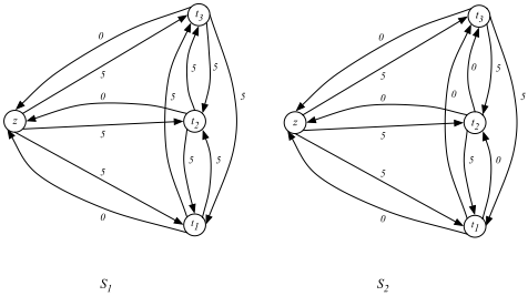
Note that both in S1 and in S2, for each i ∈ {1, 2, 3}, est(ti) = 0 and lst(ti) = 5. Hence,
So, according to the measure flexN , S1 and S2 have the same flexibility, which, of course, is counterintuitive: For each event ti in S1 we can determine its starting time between 0 and 5 independently from the other events. So, the total flexibility, expressed as the amount of choice we have in selecting a starting time for an event equals 5×3 = 15. The choice for the starting time of an event ti+1 in S2, however, may influence the choice of the starting time of the next event ti. More precisely, if (v3, v2, v1) are the latest starting times for the 3 events in S2, it is clear that 0 ≤ v3 ≤ v2 ≤ v1 = 5. Hence, the flexibility of t3 is v3 - 0, the flexibility of t2 is v2 - v3 and the flexibility of t1 is 5 - v2. So, the total flexibility of S2 equals
Therefore, the flexibility of S2 should come out as only 13 of the flexibility of S1. Generalising S1 and S2 to systems containing k concurrent and sequential events, respectively, we see that the freedom to schedule in S1 equals flex(S1) = 5 × k, while the flexibility of S2 is independent of k and remains flex(S2) = 5. Hence, if k goes to infinity, the ratio of the real flexibilities of S1 and S2 goes to infinity:
while their ratio according to flexN is exactly 1:
We conclude that the flexN metric seriously overestimates the flexibility of STNs similar to S2.
Using Upper and Lower Bounds for Every Pair of Events One reason flexN fails is that it is not able to deal with correlations between timed events. To overcome this disadvantage, we have to incorporate information about the correlation between two events as has been proposed in the definition of flexibility by Hunsberger [Hunsberger, 2002] and others [Policella et al., 2007]. Hunsberger defined his flexibility metric, which we will denote by flexH(S), by taking into account not only the apparent flexibility lst(t)-est(t) of every event t, but also the flexibility between pairs of events ti and tj. Since the distance matrix DS contains the entries DS[i, j] and DS[j, i] such that -DS[j, i] ≤ tj - ti ≤ DS[i, j] are the strongest constraints implied by C w.r.t. the temporal difference tj - ti, we can define the flexibility associated with this difference as the length of the corresponding interval 3 :
Now the flexibility of the system S can be defined by taking flexN(S) and adding to it the sum of all these flexibilities for every distinct pair of time-points, 4 i.e.,
If there is a correlation between two events ti and tj, this will result in a lower value of DS[i, j]+DS[j, i]. Hence, correlation among time events will have an influence on flexH. Although this metric is an improvement w.r.t. the naive metric flexN, the next example shows that flexH also has its shortcomings.
Example 3. Consider again the STNs S1 and S2 in Figure 1. According to flexH, the flexibility of S1 equals 3 × 5 + 3 × 10 = 45, while the flexibility of S2 equals 3 × 5 + 3 × 5 = 30. So, according to the Hunsberger metric, S2 would have a flexibility equal to 2 3 of the flexibility of S1. This seems to be an improvement with respect to the previous flexibility metric flexN assigning the same flexibility to S1 and S2. However, generalising S1 and S2 to systems containing k concurrent and sequential events, respectively, we see that
while
This means that for larger values of k, the ratio between flexH(S1) and flexH(S2) converges to 2:
while the ratio of the real flexibilities of S1 and S2 (see the previous example) goes to infinity if k goes to infinity. So, this metric is also not able to capture the correlations between the flexibilities of events in a satisfactory way.
3 Although Hunsberger defined the inverse of flexibility, i.e., rigidity of an STN, that is not relevant for our discussion at hand, since we assume a finite time horizon for an STN.
4 Actually, Hunsberger took the square root of the sum of the squares of these flexibility measures per pair, divided by (n × (n - 1)/2), the total number of different pairs of time-points.
3.1 Towards a Suitable FlexibilityMetric
Analysing the failure of both metrics flexN(S) and flexH(S) to capture the real flexibility of an STN S quickly reveals the main shortcoming of both of them: they do not fully capture the correlations between the allowed schedule-time intervals for the events t, if such correlations do exist. Considering again the system S1 (see Figure 1), it can be observed that the real flexibility can be computed by taking the sum flex(t) = flexN(t) of each event. This latter flexibility is simply determined as the difference between the latest starting time and the earliest starting time of such an event. But, as we have seen before, as soon as the events are correlated (as in the STN S2), this no longer holds, because the starting time that can be chosen for an event t is dependent upon the starting times that were chosen for other events t′ ∈ T .
So, in order to compute the flexibility of a system S, the flexibility measure should be based upon uncorrelated starting time intervals.
Definition 1. Given an STN S = (T, C), a set IS = {[lt, ut] | t ∈ T} of (non-empty) intervals for the variables in T is uncorrelated iff for every t ∈ T and every vt ∈ [lt, ut], the assignment σ, defined by σ(t) = vt, is a schedule for S.
Then, to compute the real flexibility of a system S = (T, C), we have to determine
- a set IS of uncorrelated starting time intervals [lt, ut], such that
- the sumof the interval lengths Σt∈T (ut-lt) is maximal.
This bears resemblance to the concept of safe networks discussed by [Morris et al., 2001], however, instead of tightening requirement constraints to ensure they do not affect contingent constraints, all tasks are restricted to start in an uncorrelated interval, ensuring they never affect each other.
The idea we will now pursue is to transform an STN S to an STN S′ in which new variables t-i and t+i occur for every ti ∈ T. The intuitive meaning of these variables is that they constitute the earliest and latest starting times of ti in a set IS of uncorrelated intervals.
Next, we determine the maximum flexibility of S using an LP-formulation to find a maximal solution satisfying both requirements.
Let's start with the first step. In order to ensure that the variables t-i and t+i correspond to their intended meaning, the following proposition shows how to obtain a set of uncorrelated intervals. Intuitively, this proposition states that if there exists a constraint on some tj - ti in C, then the intervals for these events should be constrained so that, within their respective intervals, the events can not be scheduled so far apart as to violate the constraint:
Proposition 2. Let S = (T,C) be an STN. A set IS = {[lti , uti ] | ti ∈ T} of intervals for the variables in T is uncorrelated if for every pair (ti, tj) ∈ T 2 , it holds that tj - ti ≤ cji ∈ C implies utj - lti ≤ cji.
Proof. Suppose the implication holds for every pair of variables. We have to show that IS is uncorrelated. So, for every t ∈ T, choose an arbitrary value vt ∈ [lt, ut] and let σ be defined by σ(t) = vt, for all t ∈ T . We now prove that σ is a schedule for S. Suppose σ is not a schedule, meaning that σ violates some constraint in C. Then there exists a constraint tj -ti ≤ cji ∈ C while σ(tj)-σ(ti) > cji. But this implies that cji < vtj - vti < utj - lti , hence utj - lti > cji, contradicting the fact that utj -ltj ≤ cji (as we have assumed to be implied by tj - ti ≤ cji ∈ C).
We will now show how to construct an STN in which the interval-endpoints are variables and the required constraints are imposed, so that, if we solve this derived STN, we are guaranteed suitable interval-endpoints:
Proposition 3. Let S = (T,C) be an STN. Consider the STN S′ = (T ′ , C′ ) derived from S as follows:
Then, for every solution σ of S′ , the set {[σ(t-), σ(t+)] | t ∈ T} is an uncorrelated set of solution intervals for S.
Proof. If C contains a constraint of the form tj - ti ≤ cji, then by the specification of the first group of constraints in C ′ , any assignment σ : T ′ → R≥0 that satisfies these constraints, also satisfies σ(t+j ) - σ(t-i ) ≤ cji, as required in Proposition 2.
Example 4. Consider the STN S2 presented in Example 1. Let STN S′2 = (T ′ , C′ ) be the transformed STN where
One possible solution is σ(t+1 ) = 4, σ(t+2 ) = 3 and σ(t+3 ) = 1, while σ(t-1 ) = 3, σ(t-2 ) = 1 and σ(t-3 ) = 0. This results in the following set of uncorrelated solution intervals: σI (t3) = [0, 1], σI (t2) = [1, 3], σI (t1) = [3, 4].
Although our transformation of S into S′ now provides an uncorrelated set of intervals, it is still insufficient to determine the flexibility of S, since the sum of the sizes of these intervals does not need to be maximal. To obtain the flexibility measure, we have to select those solutions σ for S′ that maximise the sum of the sizes of the intervals. It is easy to see that the following LP formulation will solve this problem:
Theorem 1. Let S = (T,C) be an STN. Then flex(S) can be computed by solving the following Linear Program:
As an easy consequence of these results we have the following corollary.
Corollary 1. Given an STN S = (T,C), the flexibility metric flex determines an assignment flex(t) = [t-, t+], such that for every t ∈ T and every vt ∈ [t-, t+], the assignment σ(t) = vt is a fixed-time schedule for S, satisfying all constraints in C.
Example 5. Applying the flexibility metric flex to the STNs S1 and S2 results in the following flex functions:
- For S1, we have flex(ti) = [0, 5] for i = 1, 2, 3 and flex (S1) = 3 × 5 = 15.
- For S2, we have flex(S2) = 5; one possible flex function is flex (t1) = [0, 5], flex (t2) = flex (t3) = [5, 5].
So as intended, this flexibility function will assign 3×5 flexibility units to S1, while assigning 5 units to S2.
4 DecouplingWithout Loss of Flexibility
STNs might also be used in a distributive scheduling context (see [Hunsberger, 2002; Boerkoel and Durfee, 2011; 2012; Brambilla, 2010]. Suppose that the events in T are distributed over k agents A1, . . . ,Ak such that each agent is responsible for scheduling a disjoint subset Tk ⊆ T - {z} of events. These agents act as distributed autonomous schedulers, so each agent Ai wants to determine its own schedule σi : Ti → R≥0 for the STP Si = (Ti ∪ {z},C′ i ), where Ti is the subset of tasks (time-points) assigned to Ai and C ′ i = Ti 2 ∩C is a set of constraints restricted to the events in Ti. In allowing agents to schedule autonomously, we have to ensure that no matter what choices the individual agents make in composing their individual schedule, all constraints in C are satisfied. That is, the merge σ = ⋃ki=1 σi of these individual schedules should always constitute a valid total schedule to the original problem. This problem is known as the so-called Temporal Decoupling Problem [Hunsberger, 2002].
Definition 2. Let S = (T,C) be a consistent STN. Suppose that T\{z} = {Ti}ki=1 is partitioned in k subsets Ti. Then the temporal decoupling problem is to find k STPs Si = (Ti ∪ {z},C′ i ) such that, whenever σ1, . . . , σk are independently constructed schedules for the individual STPs S1, . . . , Sk, respectively, their merge σ = ⋃ki=1 σi is a schedule for the original STP S.
To achieve an arbitrary decoupling of an STN S = (T, C) where T is partitioned into blocks Ti, we have to pay attention to constraints involving events ti and tj that belong to different agents Am and An. The problem is that agents Am and An may choose schedules σm and σn, respectively, that violate inter-agent constraint ti - tj ≤ cij, by setting σm(ti) - σn(tj) > cij. Hunsberger [Hunsberger, 2002] gave an elegant solution to this temporal decoupling problem by proposing an iterative procedure that basically makes each inter-agent constraint ti - tj ≤ DS[j, i] obsolete by tightening intra-agent constraints ti - z ≤ DS[0, i] and z - tj ≤ DS[j, 0]. These tightenings consist in selecting values δi,1 and δi,2 such that
- ti - z ≤ δi,1 ≤DS[0, i],
- z - tj ≤ δi,2 ≤DS[j, 0], and
- δi,1 + δi,2 ≤DS[i, j].
If we add the new constraints ti - z ≤ δi,1 ≤ DS[0, i] and z - tj ≤ δi,2 ≤ DS[j, 0] to S while making sure that the resulting system remains consistent, the effect is that an interagent constraint ti - tj = (ti - z) + (z - tj ) ≤ δi,1 + δi,2 ≤
DS[i, j] is now implied by the new, tighter, intra-agent constraints. Hence, the inter-agent constraint can be removed from the updated STP. Applying this procedure for every nonimplied inter-agent constraint ensures that all inter-agent constraints are implied by intra-agent constraints and the resulting system is a temporal decoupling.
Example 6. Suppose that in the STNs S1 and S2 from our earlier examples, we have agents A1, A2 and A3, where Ai is responsible for scheduling ti. In S1, every inter-agent constraint -5 ≤ ti - tj ≤ 5 is already implied by the intra-agent constraints 0 ≤ ti - z ≤ 5 and 0 ≤ tj - z ≤ 5, so decoupling is already achieved. In S2, however, we can decouple by tightening the intra-agent constraints to (for example) 0 ≤ t3 - z ≤ 2, 3 ≤ t2 - z ≤ 4 and 4 ≤ t1 - z ≤ 5, so that every inter-agent constraint is implied.
An arbitrary decoupling, however, is not always what we want, since the added constraints may limit the resulting flexibilities of the subsystems Si. Hence, the sum Σki=1flex(Si) of the flexibilities of the subsystems Si could be considerably less than the flexibility flex(S) of the original system. It is a popular belief in the research community that an optimal decoupling i.e., a decoupling that would maximize the flexibilities of the subsystems, would still suffer from some flexibility loss. In the literature we are aware of (see e.g. [Hunsberger, 2002; Boerkoel and Durfee, 2011; 2012]) several experiments have been performed to measure this loss of flexibility. However, the metrics used all have been based on the flexH metric discussed above. Instead of using this metric we try to find a decoupling that maximizes the sum of the flexibilities of the induced subsystems Si, and we consider it an optimal decoupling if the ratio (Σki=1flex(Si))/flex(S) is maximal.
Contrary to the popular beliefs in the research community we will show now that
- an optimal decoupling can be obtained in O(k)-time using the flexibility metric we discussed before,
- this optimal decoupling need not affect the flexibility of the system, i.e., we have Σki=1flex(Si) = flex(S).
Proposition 4. Let {Si}ki=1 be an optimal decoupling of an STN S. Then Σki=1flex (Si) = flex (S).
Proof. Consider the set of intervals {[lt, ut] : t ∈ T} occurring as solutions of the LP (1). Given the set A = {Ai}ki=1 of k agents, let Cinter ⊂ C be the set of all inter-agent constraints. For every inter-agent constraint t - t′ ≤ c, where t occurs in Si and t′ occurs in Sj , add the constraint t-z ≤ ut to Ci and add z - t′ ≤ -lt′ to Cj . We show the following.
Claim 1: The resulting systems {Si}ki=1 constitute a decoupling of S;
Claim 2: The sum of the flexibilities flex(Si) of the systems Si in the decoupling {Si}ki=1 equals flex(S).
Ad Claim 1. Suppose, on the contrary, that the merge σ of some combination of individual schedules σi, violates a constraint in C. This must be an inter-agent constraint t - t′ ≤ c where t occurs in Si and t′ occurs in Sj (i ̸= j). So σi(t) - σj(t′ ) > c, but since σi satisfies all constraints in Ci, it follows that σi(t) ≤ ut, and similarly, σj(t′ ) ≥ lt′ .
Therefore, σi(t) - σj(t) ≤ ut - lt′ . Since the constraint t+ -t′- ≤ c occurs in the LP, we also know that ut -lt′ ≤ c, so σi(t) - σj (t′ ) ≤ c, which contradicts σi(t) - σj (t′ ) > c. Ad Claim 2. By definition, we have Σki=1 flex (Si) ≤ flex (S). Let IS be a set of (uncorrelated) intervals [lt, ut] realizing maximum flexibility. For every subsystem Si = (Ti,Ci), consider the set ISi , being the restriction of IS to Ti. It is easy to see that each such set of intervals ISi constitutes a set of uncorrelated intervals, realizing maximum flexibility for Si. But then Σiflex(Si) = flex(S). Hence, there exists at least one decoupling realizing a total flexibility equal to the original flexibility flex (S).
Example 7. Consider Example 6. A decoupling for S2 realizing maximum flexibility can be created by adding the following decoupling constraints:
The sum of flexibilities of the subsystems equals the flexibility of the original system.
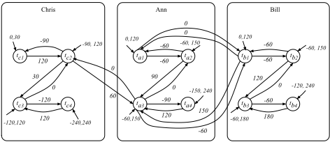
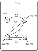
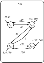
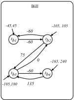
Example 8. To illustrate the difference between the current approach and previous approaches to flexibility and decoupling, we apply our method to the following STN (see Figure 2 adapted from [Boerkoel, 2012]): The STN models the activities and their constraints for three agents Chris, Ann and Bill. The purpose of this example is to show how to apply decoupling in a real-life situation, where each of the agents should have enough freedom to schedule its own activities. The flexibility of the STN S according to the flexN metric is 780 (minutes). Due to several dependencies this is a serious overestimation of the real flexibility of the system, which according to our metric equals flex(S) = 180 (minutes). In Figure 3, the result of decoupling the STN according to Boerkoel has been depicted. If this decoupling would have been optimal, we would expect its total flexibility to be equal to 180. However, the sum of the flexibilities of the three subsystems equals 135. Hence, we conclude that the decoupling applied can be improved by using our flexibility approach.
5 Conclusion and Discussion
In this paper we have discussed an efficient method to determine the flexibility of a schedule for an STN. The advantage of the flexibility metric we propose is twofold: First of all, this metric takes into account the correlations between time events unlike previous methods that have been proposed in the literature. As a consequence, our metric does not suffer from overestimations of the flexibility in an STN. Secondly, using this improved flexibility metric allows us to disprove a rather widespread belief in the research community, i.e., that temporal decoupling of an STN necessarily results in reduced flexibility: We showed that once the flexibility of an STN is determined, it can be used to decide upon a temporal decoupling that does not affect the (total) flexibility of the system.
The total flexibility of a system, however, can be obtained in many, sometimes even quite unfair, ways. For example, preserving the total flexibility of the system could mean that a decoupling heavily favors some specific agents by giving them a lot of flexibility, while harming other agents by taking away their flexibility. To prevent this, we need to come up with fair flexibility distribution schemes as an objective to grant every agent an almost equal portion of flexibility. We could propose more fair distributions of flexibility and evaluate their performance by comparing it to the maximally obtainable flexibility as we have proposed in our paper to establish the price of fairness.
Another question we did not deal with in this paper is how we should distribute flexibility over the events in order to ensure that a given interval schedule as proposed in this paper could enhance the robustness of a schedule. For example, if certain events are considered as critical or more susceptible to delays, we could try to provide them with a larger scheduling interval. Research in this direction also should pay attention to the dependencies of events upon other events (as expressed by the STN) to minimize scheduling violations. Together with extensions of the STN framework with stochastic interpretations of the upper bounds cij on the constraints, this would enable stochastic interpretations of the total flexibility of an STN and encourage empirical research into optimal distributions of flexibility over the events in order to ensure maximal (expected) robustness of the resulting schedule.
Finally, note that temporal decoupling is now done off-line before the execution of the schedule. It would be quite interesting to come up with dynamic variants of decoupling where, based on the completion times of tasks already completed, the current decoupling is adapted to profit from flexibility in an even better way.
@inproceedings{ijcai2013p356,
  title     = {Flexibility and Decoupling in the Simple Temporal Problem},
  author    = {Wilson, Michel and Klos, Tomas and Witteveen, Cees and Huisman, Bob},
  booktitle = {Proceedings of the Twenty-Third International Joint Conference on
               Artificial Intelligence, {IJCAI-13}},
  publisher = {AAAI Press / International Joint Conferences on Artificial Intelligence},
  editor    = {Francesca Rossi},
  pages     = {2422--2427},
  year      = {2013},
  month     = {8},
  url       = {https://ijcai.org/proceedings/2013/356},
}
TY - CPAPER TI - Flexibility and Decoupling in the Simple Temporal Problem AU - Wilson, Michel AU - Klos, Tomas AU - Witteveen, Cees AU - Huisman, Bob T2 - Proceedings of the Twenty-Third International Joint Conference on Artificial Intelligence, IJCAI-13 PB - AAAI Press / International Joint Conferences on Artificial Intelligence PY - 2013 SP - 2422 EP - 2427 UR - https://ijcai.org/proceedings/2013/356 ER -Copied
Machine-readable versions of this paper, for tools and AI agents:





