
Run-Time Improvement of Point-Based POMDP Policies
Proceedings of the Twenty-Third International Joint Conference on Artificial Intelligence. Pages 2408-2413.
© 2013 International Joint Conferences on Artificial Intelligence
Abstract
The most successful recent approaches to partially observable Markov decision problem (POMDP) solving have largely been point-based approximation algorithms. These work by selecting a finite number of belief points, computing alpha-vectors for those points, and using the resulting policy everywhere. However, if during execution the belief state is far from the points, there is no guarantee that the policy will be good. This case occurs either when the points are chosen poorly or there are too few points to capture the whole optimal policy, for example in domains where there are many low probability transitions, such as faults or exogenous events. In this paper we explore the use of an on-line plan repair approach to overcome this difficulty. The idea is to split computation between off-line plan creation and, if necessary, on-line plan repair. We evaluate a variety of heuristics used to determine when plan repair might be useful, and then repair the plan by sampling a small number of additional belief points and recomputing the policy. We show in several domains that the approach is more effective than either off-line planning alone even with much more computation time, or a purely on-line planning based on forward search. We also show that the overhead of checking the heuristics is very small when replanning is unnecessary.
- [Cassandra et al., 1994] Anthony R. Cassandra, Leslie Pack Kaelbling, and Michael L. Littman. Acting optimally in partially observable stochastic domains. In AAAI'94: Pro- ceedings of the Twelfth National Conference on Artificial Intelligence (vol. 2), pages 1023-1028, Menlo Park, CA, USA, 1994. American Association for Artificial Intelli- gence.
- [Kurniawati et al., 2008] H. Kurniawati, D. Hsu, and W. S. Lee. SARSOP: Efficient point-based POMDP planning by approximating optimally reachable belief spaces. In Proc. Robotics: Science and Systems, 2008.
- [Maniloff and Gmytrasiewicz, 2011] Diego Maniloff and Pi- otr Gmytrasiewicz. Hybrid Value Iteration for POMDPs. In Proceedings of Twenty-Fourth International FLAIRS Conference, 2011.
- [Pineau et al., 2006] Joelle Pineau, Geoffrey Gordon, and Sebastian Thrun. Anytime point-based approximations for large POMDPs. Journal of Artificial Intelligence Re- search, 27:335-380, 2006.
- [Ross and Chaib-draa, 2007] Stéphane Ross and Brahim Chaib-draa. AEMS: An anytime online search algorithm for approximate policy refinement in large POMDPs. In Proceedings of the 20th International Joint Conference on Artificial Intelligence, IJCAI, pages 2592-2598, 2007. IJCAI
- [Ross et al., 2008] Stéphane Ross, Joelle Pineau, Sébastien Paquet, and Brahim Chaib-draa. Online planning algo- rithms for POMDPs. Journal of Artificial Intelligence Re- search, 2008.
- [Sanner and Youn, 2011] Scott Sanner and Sungwook Youn. The Seventh international planning competition, Uncer- tainty track, 2011. 21st International Conference on Auto- mated Planning and Scheduling, Freiburg, Germany.
- [Shani et al., 2005] Guy Shani, Ronen I. Brafman, and Solomon E. Shimony. Adaptation for changing stochastic environments through online POMDP policy learning. In Workshop on Reinforcement Learning in Non-Stationary Environments, ECML, 2005.
- [Smith and Simmons, 2004] Trey Smith and Reid Simmons. Heuristic search value iteration for POMDPs. In Pro- ceedings of the 20th Conference on Uncertainty in Arti- ficial Intelligence, UAI, pages 520-527, Arlington, Vir- ginia, United States, 2004. AUAI Press.
- [Smith and Simmons, 2005] Trey Smith and Reid G. Sim- mons. Point-based POMDP algorithms: Improved analy- sis and implementation. In Proc. Int. Conf. on Uncertainty in Artificial Intelligence (UAI), 2005.
- [Sondik, 1971] Edward Jay Sondik. The Optimal Control of Partially Observable Markov Processes. PhD thesis, Stan- ford University, 1971.
- [Spaan and Vlassis, 2005] M. Spaan and N. Vlassis. Perseus: Randomized point-based value iteration for POMDPs. Journal of Artificial Intelligence Research (JAIR), pages 195-220, 2005.
- [Wang, 2013] Minlue Wang. Monitoring Plan Execution in Partially Observable Stochastic Worlds. PhD thesis, Uni- versity of Birmingham, 2013.
References were extracted automatically from the PDF and may contain errors.
Full text extracted automatically from the PDF; figures, tables and equations may differ. The PDF is the version of record.
1 Introduction
Partially observable Markov decision processes (POMDPs) [Sondik, 1971; Cassandra et al., 1994] are powerful models for sequential decision making under state and action uncertainty and have been widely investigated in the last decades. Finding optimal policies for large POMDPs is intractable because the optimal policy is a mapping over the belief space, an n - 1 dimensional continuous space if there are n states in the planning domain. Forward search-based approaches are similarly hampered because the number of possible action and observation combinations grows doubly exponentially with the planning horizon. Value iteration algorithms [Sondik, 1971] are the most popular approach to solving POMDPs. Since exact update in the entire belief state space is impractical, many approximation algorithms have been introduced that sacrifice plan quality in return for generating policies in reasonable time.
The most successful aproximation technique for POMDPs is the point-based approach (see Section 2), with point-based value iteration [Pineau et al., 2006], Perseus [Spaan and Vlassis, 2005], and SARSOP [Kurniawati et al., 2008] being widely used. All these rely on the idea of finding optimal policies in a representative belief space which is finite-a set of sampled belief points-rather than in the entire continuous belief space. All the algorithms generate policies offline that are based on the sampled belief points. However, since the value for belief points other than those sampled is interpolated from the sample points, the policies can be much worse for points far from the sampled ones. Since the full belief space is too large to be densely sampled, many pointbased algorithms choose sample points with a high probability of being reached and ignore less likely belief points. While this approach works well in many domains, it works poorly in domains where there are many low probability action outcomes-for example domains with exogenous actions, or where numerous low probability faults can occur. In these cases it is likely that execution of the policy will result in belief states for which no nearby belief point exists, and thus an arbitrarily bad policy may be followed.
As an example of the problem, consider the task of driving across a busy city, adapting the route based on observations collected en-route and radio traffic reports. Now imagine that we get evidence that a very low probability event such as a flat tyre has occcured. If there is no belief point similar to our state after this evidence, the planner will follow the best policy for an existing belief point, which may well be to continue driving to the destination. Replacing the tyre will not be considered because this action doesn't appear in the policy for any of the planned-for belief states.
The approach we take to overcome this problemdescribed in Section 3-is to use a point-based algorithm to generate an initial policy and to repair the policy at runtime by sampling a small number of additional belief points and updating the policy. The idea is that rather than doing a large amount of computation off-line, and then just looking up the policy on-line, we do significantly less computation initially, but spend some of it during the on-line phase repairing the plan. To keep this to a minimum, we evaluate a variety of cheap to compute heuristics to estimate when we may have entered a belief state for which the existing policy will perform poorly. Although exact backups are computational expensive at run-time [Shani et al., 2005], by only performing plan-repair when necessary we require significantly less execution-time computation than other on-line solvers which compute the current best course of the action at every time step. Section 4 shows our experimental evaluation of the approach.
2 POMDPs and Point-Based Algorithms
Formally, a POMDP is a tuple 〈S, A, T, Ω, O, R, β〉 where:
- S is the state space of the problem. We assume all states are discrete.
- A is the set of actions available to the agent.
- T is the transition function that describes the effects of the actions. We write T(s, a, s′ ) where s, s′ ∈ S, a ∈ A for the probability that executing action a in state s leaves the system in state s′ .
- Ω is the set of possible observations that the agent can make.
- O is the observation function that describes what is observed when an action is performed. We write O(s, a, s′ , o) where s, s′ ∈ S, a ∈ A, o ∈ Ω for the probability that observation o is seen when action a is executed in state s resulting in state s′ .
- R is the reward function that defines the value to the agent of particular activities. We write R(s, a) where s ∈ S, a ∈ A for the reward the agent receives for executing action a in state s.
- β is a discount factor.
POMDPs differ from MDPs in that they need to estimate the current state rather than knowing exactly which state the agent is in. That is, they need to maintain a belief state, a distribution over S calculated from the initial belief state and the history of actions and observations. Given this, a policy for a POMDP is a mapping from belief states to actions.
One way of representing the value of a policy is as a set of |S|-dimensional hyper-planes called α-vectors, which are piece-wise linear and convex [Sondik, 1971]. The goal of value iteration algorithms is to find those α-vectors so that the best policy π∗ can be derived as:
where each α-vector defines the expected future reward, starting with action a and then continuing to execute the action with the highest α-vector in subsequent belief states.
To compute optimal α-vectors, one of the key operators in POMDP solvers is to build n-horizon value functions from n - 1-horizon ones using the backup operator H:
where P (o|a, b) = ∑s,s′∈S O(s, a, s, o)b(s)T (s, a, s′ ) is the probability of getting observation o when doing action a in belief state b. For each observation o, there is only one deterministic transition from the current belief state b to a new belief state b′ , which can be computed via Bayes rule.
Since the belief space is continuous and high-dimensional, generating α-vectors over the entire space is computational expensive. However, the computation time of the backup operation for a single belief point is O(|S|2 |A||O||Vn-1|), which takes only polynomial time. Point-based value iteration was introduced to take advantage of this by planning in a representative subset of the belief space.
Point-based value iteration (PBVI) [Pineau et al., 2006] maintains one α-vector per point, so the number of α-vectors is never greater than the number of belief points. In the backup stage, updates of α-vectors are only performed on this representative set of belief points. By doing so, [Pineau et al., 2006] performs a full point-based update in polynomial time and the size of the value function remains constant. To construct the belief point set, PBVI stochastically simulates forward trajectories for belief points already in B and greedily adds the belief point which is furthest away from the existing belief set to B.
The Perseus algorithm [Spaan and Vlassis, 2005] differs from PBVI in belief point generation strategy and backup strategy. It first explore the world with a random walk to generate an initial belief points set B. It then calulates the value function for these belief points, but in each backup it also marks all other belief points that are improved by the new α-vector, and then backs up an unmarked point. By doing so, the number of backup operations can be reduced at each iteration.
Perseus and PBVI use vector representations for value functions which are a lower bound on the optimal value function. Heuristic search value iteration (HSVI) [Smith and Simmons, 2004; 2005] uses both lower and upper bounds. The lower bounds are again represented as α-vectors and upper bounds are represented as a point set where each point stores the belief value and its upper bound value. Instead of updating upper bounds and lower bounds for each belief point at each iteration, HSVI firstly perform a heuristic search to explore new belief points. When the search is completed by satisfying a termination condition, such as thresholding the difference between the lower and upper bound, backup operations are executed from the newly generated belief points to the initial belief point.
SARSOP [Kurniawati et al., 2008] also uses lower and upper bounds but it attempts to generate belief points which are in the optimal reachable region at the belief point sampling stage by alternating between sampling new belief points and backup operations to update the bounds. Pruning techniques are also applied to remove dominated α-vectors. By computing the values as the points are generated, the points chosen are not just reachable as in the other point based algorithms but are reachable when following the discovered policy.
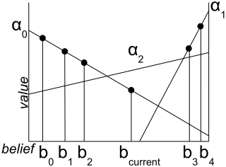
At run time, point-based algorithms compute the best αvector from the vector set for the current belief point at each time step, but if the current belief point has no closeby belief points, its performance is likely to be poor. Figure 1 shows a set of α vectors and the belief point set B = {b0, b1, b2, b3, b4} from which it was generated. As we can see from the figure, B only leads to two α-vectors α0 and α1. As the current belief point bcurrent diverges from any of the points we use to generate the vectors, these vectors are increasingly unlikely to be optimal. For example, there might be a potential better vector α2 for our current belief point.
The alternative to the off-line POMDP solvers described above is to plan on-line from the current belief state at every step (see [Ross et al., 2008] for a survey of on-line techniques). On-line solutions generally generate a rough policy off-line, for example using PBVI, as in [Ross and Chaib-draa, 2007], and then use local search at run-time to improve this. Most recent algorithms use the off-line policy to generate a heuristic that is then used to guide heuristic search on-line. This approach has two disadvantages. First, the same amount of computation is used at run-time whether the belief state is close to those used to generate the initial policy or is far away. Second the heuristic remains fixed, so the computation used in calculating the best action from one belief state provides no benefit when calculating the best action at future belief states. Hybrid POMDP [Maniloff and Gmytrasiewicz, 2011] attempted to solve the second problem by at each step deciding whether to spend a small portion of the on-line computation on improving the initial policy so later search can benefit. However, they base their decisions on very approximate lower and upper bounds on the value function. The approach we describe below can be thought of as a way to overcome both the above disadvantages. We spend more time on the initial policy than an on-line algorithm might, so our initial policy is hopefully better, and we then use heuristics to decide when to simply rely on the current policy and when to do extra computation to improve it, but unlike the on-line approaches we re-use the extra computation in future by incorporating its results into the off-line generated policy.
One final piece of related work is [Shani et al., 2005], which proposes an online POMDP learning algorithm which can adapt for slow environment change. While this does update the off-line policy in a way similar to ours, its different motivation (a changing model, rather than poor approximation) leads to a rather different solution.
Algorithm 1 Execution Monitoring on PBVI
Let b be the initial belief state Let B be the sampled belief point set from off-line SARSOP generation. Let V be the set of α-vectors from off-line SARSOP generation. Let ¯ V be the pair of belief point and its upper value from off-line SARSOP generation. Set θ and τ where θ is the threshold value for triggering replanning and τ is the replanning time constraint. repeat V )
if Measurement(b, B) > θ then V ← ¯ V ′ end if execute from V until reach of plan horizon3 Plan Repair for Point-Based Policies
As explained in the previous section, at each time step traditional point-based algorithms simply compute the best αvector from the approximate solution for the current belief point and ignore the question of whether the current suboptimal solution is good enough or not. In this section we describe our approach for detecting when this is unlikely to be optimal and repairing the policy.
There are two parts in our plan repair strategy. The first is execution monitoring, in which we use a heuristic to estimate when the current best solution may not be very good. We propose four different heuristic measures, each of which is relatively cheap to compute-they need to be as they will be computed after every action-and hopefully provides useful information about when the policy may be poor, and also examine combinations of measures. In each case, we simply apply a threshold θ on the heuristic value of a belief state to decide when to trigger replanning.
The second part of our plan repair strategy is replanning when our heuristic functions indicate that the current policy for our current belief point should be improved. A naive replanning from scratch would be too costly. Instead, we treat the current belief point as a new initial state, use the already computed lower and upper bounds provided by the previous invocation of SARSOP, and ask SARSOP to generate new belief points and a new policy. To do this we not only need to store belief points from the off-line stage, but we also need to keep a record of the upper bounds of the optimal policythe set of belief points and their upper values. Newly generated belief points will be added to the existing belief point set which can be used for determining the quality of the policy for subsequently encountered belief points. As well, new lower bounds and upper bounds are computed as part of replanning. We limit the time available to SARSOP to prevent replanning taking too long. The plan repair algorithm is displayed in Algorithm 1.
We now describe the several candidate heuristics, and compare their performance in Section 4.
Gap heuristic
The first heuristic function is using the gap between upper bound and lower bound of current belief point b as shown in Eq 4. However, this heuristic function only works with the point-based algorithms that generate both upper bounds and lower bounds such as SARSOP but does not suitable for all point-based algorithms. Therefore, we also proposed other heuristic functions that can work on general point-based algorithms. The time complexity of this heuristic is O(|Γ|) where Γ is the set of α vectors.
L1 Distance
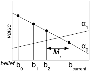
The second heuristic we use is simply the L1 distance from bcurrent to the nearest point in B where B is the current belief point set. Intuitively, if the current belief point is far away from any points that are used to generate the initial policy, it is quite likely that we can find some better α vectors for the current belief. Figure 2 demonstrates this idea. b0, b1, b2 and bcurrent share the same best α-vector. We use an L1 metric to measure the distance between the points, so in this case the distance between bcurrent and b2 is computed to make a decision about whether to trigger plan repair. The time complexity of this function is O(|B|).
Formally, the L1 heuristic for approximating the value function error at some belief point b given belief point set B is computed as follows:
If M1(b,B) ≥ θ, we execute our replanning operations where θ is the pre-defined threshold parameter.
Value Difference
The third heuristic we propose is based on the difference between the value of the best α-vector at b and the average value of all the belief points Bα that share the same best α-vector. To produce a scale-invariant heuristic we divide this difference by the average value of the belief points that share the same best α-vector. This is again thresholded to trigger plan repair. Figure 3 illustrates this second heuristic measurement. Our current belief point bcurrent shares the same α-vector α0
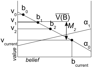
with belief points b0, b1 and b2. The intuition is that since the current belief point shares the same α-vectors with these points, it should come from a similar region of the belief space and should have a similar value. Therefore, the average value of belief points b0, b1 and b2 is computed as vaverage and compared with current value vcurrent. Figure 3 shows that the current belief point's value is far from the average of the other points and possibly indicates there is a need for replanning.
Formally, the lower bound value measurement is computed as follows:
where Vα(B) is the average value of all belief points which have the same best α-vector as point b. The complexity is O(|Bα||Γ|).
Belief Point Entropy and Number of Iterations
We observe that in addition to the proposed distance measures above there are two other factors which affect the overall performance of the execution of the POMDP policy. One is the number of times we have triggered our replanning during plan execution. The second factor is the entropy of the belief point-we find that when the current belief point has larger entropy, it often leads to a bigger improvement from replanning compared to ones with small entropy. One explanation could be that belief points with less entropy are less uncertainty and more likely to be in the corners of the belief space and have already been covered by the initial upper and lower bounds generated by SARSOP.
These two factors are not related to the sampled belief points set but can be seen as independent properties that will affect our overall performance. We combine the previous two heuristics with these two additional factors to form another two heuristic functions as follows (β and γ are weights for combining the two factors):
| Factory (54s, 6a, 2o) | Gen. & Exec. Time (s) | Total Reward |
|---|---|---|
| SARSOP (no replanning) | 400 + 0.01 | 286.68 ± 213.56 |
| SARSOP (no replanning) | 200 + 0.01 | 280.41 ± 220.88 |
| SARSOP (no replanning) | 100 + 0.01 | 292.6 ± 229.9 |
| Random Replan | 100 + 8.56 | 452.4 ± 201.9 |
| Gap | 100 + 0.32 | 261.7 ± 218.6 |
| Gap | 100 + 1449.8 | 589.5 ± 115.5 |
| Heuristic M1 | 100 + 5.64 | 566.2 ± 81.7 |
| Heuristic M2 | 100 + 3.09 | 581.2 ± 70.6 |
| Heuristic M3 | 100 + 10.21 | 602.8 ± 3.0 |
| Heuristic M4 | 100 + 3.93 | 608.3 ± 48.3 |
| look-ahead (blind strategy) | 0.06 + 3.5 | 240.8 ± 192.7 |
| look-ahead (SARSOP offline) | 100 + 343.9 | 611.9 ± 28.4 |
Again, β and γ are used to weight the components of the heuristic. As we describe in the next section, we systematically varied them for each domain and choose "standard" values that work reasonably well for all the domains. The complexity of M3 and M4 are O(|S|+|B|) and O(|S|+|Bα||Γ|) respectively.
4 Experiments
There are several possible models for dividing computation between on- and off-line. We don't commit to a particular one here, but instead try to maximise policy quality while minimising total computation. The experiments are designed to evaluate the plan repair strategy compared with SARSOP, and to compare the heuristics in a number of domains.
We test our approach on three POMDP domains chosen to have the characteristics under which the approach should be particularly effective. The first is a factory domain where the goal is to successfully assemble a product using a number of robotic arms. Each of the arms can be in one of three states, either ON, OFF or FAULTY. The TurnOn action makes an arm transition from the OFF state to the ON state. The Assemble action is used to assemble the product, but requires that all the arms are turned on before it will succeed. In addition, with a low probability (0.001), when we execute the Assemble action, all the arms become faulty. There is also a repair action for each arm which can recover the arm from the FAULTY state to the OFF state. Executing the Assemble action results in a positive reward if all the arms are ON, and no reward if any arm is not ON. Noisy observations of arm state are available only when we execute the Assemble action.
The second domain is the reconnaissance domain from the International Planning Competition [Sanner and Youn, 2011], where an agent is equipped with tools such as water detectors, life detectors and cameras. A positive reward is given when the agent takes pictures at a place which has water and life. The sensing actions are noisy which means a trade-off between the cost of the sensing actions and the information gained from the sensing actions needs to be made. There are also some hazardous locations where the agent's equipment has a 0.01 probability to become damaged if it enters them. If the equipment is damaged, the agent needs to return to the base where it can apply repair actions. In the original version of this domain the state of all tools is observed at every step. We modify this assumption so that only when we move out of the hazardous places do we make observations about the status of the equipment.
| Reconnaissance (4096s, 14a, 8o) | Gen. & Exec. Time (s) | Total Reward |
|---|---|---|
| SARSOP (no replanning) | 400 + 1.48 | 1730.4 ± 1382.0 |
| SARSOP (no replanning) | 200 + 1.09 | 1559.5 ± 1279.0 |
| SARSOP (no replanning) | 100 + 0.58 | 1507.3 ± 1244.9 |
| Random Replan | 100 + 21.11 | 2981.7 ± 871.8 |
| Gap | 100 + 14.73 | 3493.9 ± 584.7 |
| Heuristic M1 | 100 + 17.51 | 3597.2 ± 305.2 |
| Heuristic M2 | 100 + 11.14 | 3325.9 ± 864.6 |
| Heuristic M3 | 100 + 17.28 | 3530.0 ± 1045.6 |
| Heuristic M4 | 100 + 7.09 | 3357.5 ± 890.8 |
| look-ahead (blind strategy) | 22.75 + 295.9 | 469.6 ± 421.2 |
| look-ahead (SARSOP offline) | 100 + 1281.9 | 3698.5 ± 309.8 |
The third domain is a modified version of reconnaissance domain. Because there is only one repair action for each tool in the second domain, we add one more repair action for each equipment to make the domain more complex. The two repair actions have different accuracy and costs 1 .
Results
The five heuristic measurements and straight SARSOP are tested on the three domains. Two general parameters are considered here. One is the threshold θ, which is used for determining whether the current policy is good enough for the current belief point. The other is the replanning time τ , which is applied as a time constraint for replanning. We use the following function to find the best parameters for each heuristic:
where Max(Reward) is the maximum total reward and Max(T ime) is the maximum execution time. The parameter settings used were optimised over all three domains and then the same settings were used for all experiments.
In each domain we compare standard SARSOP with 100 seconds, 200 seconds, or 400 seconds available for policy generation. As well as standard SARSOP and SARSOP with our plan repair, we also run SARSOP with replanning triggered randomly. To make this a fair comparison, we first calculate the average number of replannings in each domain, where the average is over all the heuristics tested, then for the random replanning variant we set the probability of replanning at each step so the expected number of replannings is the same. We also compared our results with an on-line lookahead algorithm where the current best action is computed by expanding the search tree at each time step. Because on-line POMDP solvers require an off-line policy to provide heuristic values for each state, we show results using both a blind strategy and the policy generated by SARSOP for the heuristic.
1 Full details of the domains, as well as additional experiments and analysis can be found in [Wang, 2013]
| Modified Recon. (4096s, 16a, 8o) | Gen. & Exec. Time (s) | Total Reward |
|---|---|---|
| SARSOP (no replanning) | 400 + 0.41 | 1470.8 ± 1321.4 |
| SARSOP (no replanning) | 200 + 0.97 | 1511.1 ± 1138.8 |
| SARSOP (no replanning) | 100 + 0.78 | 1704.7 ± 1367.0 |
| Random Replan | 100 + 15.48 | 2831.3 ± 861.2 |
| Gap | 100 + 20.4 | 3185.8 ± 1120.0 |
| Heuristic M1 | 100 + 44.68 | 3152.4 ± 1122.9 |
| Heuristic M2 | 100 + 11.76 | 3491.7 ± 641.5 |
| Heuristic M3 | 100 + 18.05 | 3694.7 ± 332.5 |
| Heuristic M4 | 100 + 12.69 | 3362.8 ± 843.4 |
| look-ahead (blind strategy) | 28.7 + 625.7 | 400.4 ± 79.5 |
| look-ahead (SARSOP offline) | 100 + 272.0 | 3582.9 ± 431.1 |
The performance comparisons are displayed in Tables 1-3. Initial policies are generated by SARSOP with a time limit of 100 second, and execution time is the average CPU time for each problem over 100 trials. As the tables show, our plan repair approaches generally improves standard SARSOP in terms of total reward by more than 100% in all three domains. Even when SARSOP has four times as much computation time, our approach still performs much better, and it is clear from the SARSOP performance, particularly in the Factory domain, that further computation will not improve the policy. Random replanning does surprisingly well, largely because in these domains there is no penalty for carrying on with normal actions after a fault has occurred, so the system can keep acting badly until replanning occurs, without a penalty. The on-line algorithm using the blind strategy does not generate sensible policies, and with the SARSOP policy produces better results in total reward but also requires much more execution time. We did not inject faults into the runs, so if no fault occurs at all, all the approaches will perform very well. This is shown in the standard deviations of the rewards, which typically fall as reward increases, reflecting the fact that the replanning improves only the low reward runs.
Comparing the heuristics, we note that while the Gap heuristic works well for the two reconnaisance domains, it performs very poorly in the Factory domain, where the two different entries in the table correspond to two different thresholds for replanning. The poor performance is because it is extremely sensitive to this threshold because the noisy observations mean the belief states change only gradually from a belief that everything is OK to one in which a fault has occurred. This results in a heuristic that either doesn't replan at all, or replans far too often.
| Hallway2 | Gen. & Exec. Time (s) | Total Reward |
|---|---|---|
| SARSOP (no replanning) | 100 + 0.01 | 6.91 ± 1.95 |
| Heuristic M1 | 100 + 0.68 | 7.02 ± 1.87 |
| RockSample(4,4) | ||
| SARSOP (no replanning) | 100 + 6.43 | 1338.4 ± 208.17 |
| Heuristic M1 | 100 + 22.77 | 1343.0 ± 159.02 |
Heuristic M2 is cheaper to compute than M1 because we store the best α-vector for each point, so all that needs to be done is calculate the averages, which for domains of this size is cheaper than computing the L1 norm. There is a statistical significant difference between the performance of M3 and M4 and that of M1 and M2 for the Factory and Modified reconnaisance domains.
To show performance in domains that do not have the properties we expect to benefit our approach, we also compared with SARSOP in the Hallway2 problem (92 states) and the rock sample domain (4096 states). As shown in table 4, SARSOP does a good job of covering the policy for Hallway2 so replanning is rarely needed. On this kind of domain our approach only evaluates the heuristic at each step, so the overhead compared with standard SARSOP is small. On the rock sample domain we see a small amount of replanning and a slight improvement in performance.
5 Conclusions
Point-based POMDP solvers have in the last decade produced great improvements in solving large POMDP problems. They compute near-optimal policies by focusing on the reachable belief space but in large domains or those with many possible action outcomes may not place sufficient belief points for to cover the policy. We have presented a plan repair-based approach which can be seen as an integration of on-line and offline approaches to solve this problem. Experiments on three domains which share the same properties that some states are visited with small probability demonstrate that off-line pointbased algorithms perform poorly in these domains and our approach can perform significantly better. Results in the Hallway2 domain show that even where the initial policy is good, the overhead of plan repair is relatively small.
In all our experiments we have used total reward received as our measure of plan quality, rather than discounted reward. Discounted reward shows a much smaller effect because of the rarity that transitions to the "fault states" occur in our domains-the effects of following the bad policy tend to be enough steps in the future that their effect on the discounted reward in the initial state are negligible. However, in most cases the initial policy will never recover from these faults when they ocur, so discounted reward just before a fault occurs is much more significant. We felt using total reward was a fairer comparison than artificially inducing faults.
@inproceedings{ijcai2013p354,
  title     = {Run-Time Improvement of Point-Based POMDP Policies},
  author    = {Wang, Minlue and Dearden, Richard},
  booktitle = {Proceedings of the Twenty-Third International Joint Conference on
               Artificial Intelligence, {IJCAI-13}},
  publisher = {AAAI Press / International Joint Conferences on Artificial Intelligence},
  editor    = {Francesca Rossi},
  pages     = {2408--2413},
  year      = {2013},
  month     = {8},
  url       = {https://ijcai.org/proceedings/2013/354},
}
TY - CPAPER TI - Run-Time Improvement of Point-Based POMDP Policies AU - Wang, Minlue AU - Dearden, Richard T2 - Proceedings of the Twenty-Third International Joint Conference on Artificial Intelligence, IJCAI-13 PB - AAAI Press / International Joint Conferences on Artificial Intelligence PY - 2013 SP - 2408 EP - 2413 UR - https://ijcai.org/proceedings/2013/354 ER -Copied
Machine-readable versions of this paper, for tools and AI agents:





