
Problem Splitting Using Heuristic Search in Landmark Orderings
Proceedings of the Twenty-Third International Joint Conference on Artificial Intelligence. Pages 2401-2406.
© 2013 International Joint Conferences on Artificial Intelligence
Abstract
In this paper, we revisit the idea of splitting a planning problem into subproblems hopefully easier to solve with the help of landmark analysis. While this technique initially proposed in the first approaches related to landmarks has been outperformed by landmark-based heuristics, we believe that it is still a promising research direction. To this end, we propose a new method for problem splitting based on landmarks which has two advantages over the original technique: it is complete (if a solution exists, the algorithm finds it), and it uses the precedence relation over the landmarks in a more flexible way. We lay in this paper the foundations of a meta best-first search algorithm, which explores the landmark orderings to create subproblems and can use any embedded planner to solve subproblems. It opens up avenues for future research: among them are new heuristics for guiding the meta search towards the most promising orderings, different policies for generating subproblems, and influence of the embedded subplanner.
- [Bibaï et al., 2010] Jacques Bibaï, Pierre Savéant, Marc Schoenauer, and Vincent Vidal. An evolutionary meta- heuristic based on state decomposition for domain- independent satisficing planning. In Proceedings of the International Conference on Automated Planning and Scheduling (ICAPS), pages 18-25, 2010.
- [Bonet and Geffner, 2001] Blai Bonet and Hector Geffner. Planning as heuristic search. Artificial Intelligence, 129(1):5-33, 2001.
- [Fikes and Nilsson, 1972] Richard E. Fikes and Nils J. Nils- son. STRIPS: A new approach to the application of the- orem proving to problem solving. Artificial Intelligence, 2(3-4):189-208, 1972. IJCAI
- [Ghallab et al., 2004] Malik Ghallab, Dana Nau, and Paolo Traverso. Automated Planning, theory and practice. Morgan-Kaufmann, 2004.
- [Helmert and Domshlak, 2009] Malte Helmert and Carmel Domshlak. Landmarks, critical paths and abstractions: What's the difference anyway? In Proceedings of the International Conference on Automated Planning and Scheduling (ICAPS), 2009.
- [Hoffmann and Nebel, 2001] Jörg Hoffmann and Bernhard Nebel. The FF planning system: Fast plan generation through heuristic search. Journal of Artificial Intelligence Research, 14:253-302, 2001.
- [Hoffmann et al., 2004] Jörg Hoffmann, Julie Porteous, and Laura Sebastia. Ordered landmarks in planning. Journal of Artificial Intelligence Research, 22:215-278, 2004.
- [Keyder et al., 2010] Emil Keyder, Silvia Richter, and Malte Helmert. Sound and complete landmarks for and/or graphs. In Proceedings of the European Conference on Artificial Intelligence (ECAI), pages 335-340, 2010.
- [Kishimoto et al., 2009] Akihiro Kishimoto, Alex Fuku- naga, and Adi Botea. Scalable, parallel best-first search for optimal sequential planning. In Proceedings of the Inter- national Conference on Automated Planning and Schedul- ing (ICAPS), 2009.
- [Richter and Helmert, 2009] Silvia Richter and Malte Helmert. Preferred operators and deferred evaluation in satisficing planning. In Proceedings of the International Conference on Automated Planning and Scheduling (ICAPS), pages 273-280, 2009.
- [Richter et al., 2008] Silvia Richter, Malte Helmert, and Matthias Westphal. Landmarks revisited. In Proceedings of the 23rd AAAI Conference on Artificial Intelligence, pages 975-982, 2008.
- [Rintanen, 2012] Jussi Rintanen. Engineering efficient plan- ners with sat. In Proceedings of the European Conference on Artificial Intelligence (ECAI), pages 684-689, 2012.
- [Sebastia et al., 2006] Laura Sebastia, Eva Onaindia, and Eliseo Marzal. Decomposition of planning problems. AI Communications, 19:49-81, 2006.
- [Vernhes et al., 2013] Simon Vernhes, Vincent Vidal, and Guillaume Infantes. Landmark-based meta best-first search algorithm: First parallelization attempt and eval- uation. In Proceedings of the ICAPS-2013 Workshop on Heuristics and Search for Domain-independent Planning (HSDIP), 2013.
- [Vidal, 2004] Vincent Vidal. A lookahead strategy for heuristic search planning. In Proceedings of the Interna- tional Conference on Automated Planning and Scheduling (ICAPS), pages 150-159, 2004.
- [Vidal, 2011] Vincent Vidal. YAHSP2: Keep it simple, stupid. In Proceedings of the 7th International Planning Competition (IPC'11), 2011.
- [Zhu and Givan, 2003] Lin Zhu and Robert Givan. Land- mark extraction via planning graph propagation. In ICAPS Doctoral Consortium, pages 156-160, 2003.
References were extracted automatically from the PDF and may contain errors.
Full text extracted automatically from the PDF; figures, tables and equations may differ. The PDF is the version of record.
1 Introduction
Automated Planning in Artificial Intelligence [Ghallab et al., 2004] is a general problem solving framework which aims at finding solutions to combinatorial problems formulated with concepts such as actions, states of the world, and goals. Landmark-based analysis is actually among the most popular tools to build efficient planning systems, either optimal or suboptimal. Landmarks are facts that must be true at some point during the execution of any solution plan, and some of them can be found, as well as an ordering, in polynomial time [Hoffmann et al., 2004; Keyder et al., 2010]. Landmarks have been used in two main ways. The most successful one is the design of heuristic functions to guide search algorithms, such as the landmark-counting heuristic used in the LAMA suboptimal planner [Richter et al., 2008] or the LMCut heuristic for optimal cost-based planning [Helmert and Domshlak, 2009]. An anterior method proposed in [Hoffmann et al., 2004] is to divide a planning problem into successive subproblems whose goals are disjunctions of landmarks to be achieved in turn by any embedded planner. This method is not as efficient as using landmark-based heuristics: among the most prominent problems are its incompleteness and its lack of flexibility with respect to an initial ordering of the landmarks. STeLLa [Sebastia et al., 2006] is another problem-splitting method which creates a set of subproblems using conjunctions of landmarks.
We aim in this paper to revisit these last methods, with the objective of devising a complete algorithm for subproblem splitting based on landmarks. Roughly speaking, our method consists in performing a best-first search algorithm in the space of landmark orderings, in which node expansion implies the search of a subproblem by an embedded planner. This search algorithm is performed at a meta level, the low level being the search made by the embedded planner that can itself use a best-first search algorithm. After giving some background about classical planning and landmark computation, we define the basic components later used to describe the landmark-based meta best-first search algorithm (LMBFS), along with several heuristics to guide the meta search, and experimentally evaluate their influence on the planner efficiency. We finally conclude and present some perspectives for future works.
2 Background on Classical Planning
2.1 STRIPSModel of Planning
The basic STRIPS [Fikes and Nilsson, 1972] model of planning can be defined as follows. A state of the world is represented by a set of ground atoms. A ground action a built from a set of atoms A is a tuple 〈pre(a),add(a),del(a)〉 where pre(a) ⊆ A, add(a) ⊆ A and del(a) ⊆ A represent the preconditions, add and delete effects of a, respectively.
A planning problem is defined as a tuple Π = 〈A, O, I , G〉, where A is a finite set of atoms, O is a finite set of ground actions built from A, I ⊆ A represents the initial state, and G ⊆ A represents the goal of the problem. The application of an action a to a state s is possible if and only if pre(a) ⊆ s and the resulting state is s′ = (s \ del(a)) ∪ add(a). A solution plan is a sequence of actions 〈a1, . . . , an〉 such that for s0 = I and for all i ∈ {1, . . . , n}, the intermediate states si = (si-1 \ del(ai))∪add(ai) are such that pre(ai) ⊆ si-1 and G ⊆ sn. S(Π) denotes the set of all solution plans of Π. We also denote ◦ the concatenation of two plans, i.e. 〈a1, . . . , ai〉 ◦ 〈aj, . . . , ak〉 = 〈a1, . . . , ai, aj, . . . , ak〉.
2.2 Landmarks
Classical landmark definitions state that landmarks are facts that must be true at some point during the execution of any solution plan [Hoffmann et al., 2004; Keyder et al., 2010]. We use the following definition of landmarks:
Definition 1 (Causal landmark). [Zhu and Givan, 2003] Given a planning problem Π = 〈A,O, I,G〉, an atom l is a causal landmark for Π if either l ∈ G or ∀ρ ∈ S(Π), ∃a ∈ ρ : l ∈ pre(a).
An intuitive precedence relation among landmarks and a graph based on this relation can be defined as follows:
Definition 2 (Precedence relation <L). <L can be defined on a set of landmarks L: (∀(l, l′ ) ∈ L2 ) l <L l′ if the first occurence of l is reached before the first occurence of l′ by the execution of every solution plan.
Definition 3 (Landmark graph Γ). Given a set of landmarks L and a precedence relation <L, we define Γ = (V, E), the corresponding landmark directed graph where the set of vertices V = L and the set of edges E is the transitive reduction of the graph (V, {(l, l′ ) ∈ L2 | l <L l′ }).
Definition 4 (Relatives of a landmark l). Accordingly to the graph Γ, we denote PaΓ(l) the set of parents of l, ChΓ(l) the set of children of l, and PΓ(l) the set of ancestors of l.
We now introduce the following definitions that we will rely on. First, we denote root landmarks of a landmark graph all landmarks associated to vertices with no parents:
Definition 5 (Root landmark set). Let Γ = (V, E) be a landmark graph: roots(Γ) = {l ∈ V | PaΓ(l) = ∅}.
We now define the subgraph Γ \ A built by removing from the landmark graph Γ the vertices associated to landmarks in A and their corresponding edges:
Definition 6 (Landmark subgraph). Let Γ = (V, E) be a landmark graph and A be a set of landmarks: Γ \ A = (V \ A, {(v, v′ ) ∈ E | v /∈ A∧ v′ /∈ A}).
Landmark Graph Generation
Practicals methods proposed to produce landmark graphs [Hoffmann et al., 2004; Zhu and Givan, 2003] are based on a Relaxed Planning Graph (RPG) of Π. More complex types of landmarks might be considered [Keyder et al., 2010]. In this work, we choosed the method of [Zhu and Givan, 2003] for its simplicity.
Related Works on Using Landmarks
Previous approaches used landmarks in mainly two different ways. One approach is computing heuristics. For example, the LAMA heuristic [Richter et al., 2008] estimates a heuristic value of the states by counting unreached and required again landmarks. Another approach is to split a planning problem into subproblems. Disjunctive Search Control (DSC) [Hoffmann et al., 2004] is a search control algorithm based on the landmark graph. It runs a subplanner on the problem Π whose goal is the disjunction of the roots of the landmark graph and G. If a valid plan is found, then the reached landmark is removed from the landmark graph and the algorithm iterates (the reached state is used as the new initial state) until the landmark graph is empty. Finally, the subplanner is called a last time with G as goal.
3 The Landmark-basedMeta Best-First Search (LMBFS) Algorithm
Our approach is based on problem splitting with a flexible exploitation of the landmark graph: LMBFS performs a bestfirst search in a space of subproblems generated on-the-fly, based on possible landmark orderings.
More precisely, LMBFS builds a search tree where nodes represent planning problems that are subproblems of the original one. Solving subproblems along a branch of this tree leads to iteratively reach each landmark in a possible ordering, the initial state of each subproblem being the final state obtained by applying the plan found for the previous subproblem. We formally define in this section the metanodes and associated planning problems, as well as different ways of generating the next subproblems to solve from a metanode (the children of that metanode in the search tree). Both aspects heavily rely on the landmark graph and on the partial order it defines. We then give the complete algorithm, heuristics used and implementation details.
In the following, we consider a planning problem Π = 〈A, O, I, G〉, its corresponding set of landmarks L, and Γ the landmark graph associated to Π.
3.1 Metanode and Associated Planning Problem
We first define metanodes and associated problems:
Definition 7 (Metanode). A metanode is a tuple m = 〈s, h, A, l, ρ〉 where:
- s is a state of the planning problem Π;
- h is a heuristic evaluation of the node;
- A is a set of landmarks (A ⊆ L);
- l is a landmark (l ∈ L);
- ρ is a plan yielding the state s from the initial state I.
Definition 8 (Metanode-associated planning problem). The planning problem associated to a metanode m = 〈s, h,A, l, ρ〉 is Πm = 〈A, opsΓ(l,A), s, {l}〉 with opsΓ(l, A) a subset of O defined below.
We consider the planning problem where s is the initial state, A is the set of ground atoms of Π, {l} is the goal. In order to focus search on reaching l, we forbid the actions producing some other landmarks by defining opsΓ(l,A) as a subset of actions associated to a landmark subgraph:
Definition 9 (Landmark subgraph action restriction). Let m = 〈s, h,A, l, ρ〉 be a metanode. opsΓ(l,A) = {a ∈ O | (l ∈ add(a)) ∨ (add(a) ∩ roots(Γ \ A) = ∅)}.
In other words, opsΓ(l,A) is the set of actions producing l and actions which does not produce any root landmarks of the subgraph Γ \ A (except if they also produce l). In our algorithm, A will be the set of already achieved landmarks.
3.2 Expansion of Metanodes
There are several ways to generate children of a metanode, or equivalently defining other subproblems to solve. Let us recall that a metanode m = 〈s, h,A, l, ρ〉 defines a problem starting from s and focusing on achievement of landmark l by forbidding actions producing other landmarks of roots(Γ\A) (except if they also produce l). In the following, h′ is the heuristic evaluation of the generated metanode, discussed in section 3.4.
Next Landmarks Metanode Generation
This first metanode generator tries to follow the landmark graph Γ as closely as possible, exploring sequences from the roots to the leaves. The idea is the following: when the goal landmark of the metanode can be reached, generate children in order to reach other root landmarks in Γ. We thus define the nextLM operator as:
Definition 10 (Next landmarks metanode generation). Let m = 〈s, h,A, l, ρ〉 be a metanode. If Πm has a solution ρ′ , then nextLM(m) = {〈s′ , h′ ,A ∪ {l}, l′ , (ρ ◦ ρ′ )〉 | l′ ∈ roots(Γ \ (A ∪ {l}))} where s′ is the state obtained by applying ρ′ to s. If Πm has no solution, nextLM(m) = ∅.
In other words, at a metanode m, we try to reach the landmark l. If there is a plan, the landmark l is added to the set of already achieved landmarks A, and the partial plan is updated accordingly. Then, new metanodes are generated by looking at root landmarks in the restricted graph Γ \ (A ∪ {l}).
Remark. Using nextLM, we can explore every total order created from the precedence relation <L, which was our objective. Indeed, consider a metanode focusing on an initial root landmark of Γ. If we generate its children using the nextLM operator, then selecting one of them and iterating the process in a depth-first way, we will eventually empty the landmark graph Γ, achieving the exploration of a total order of all landmarks.
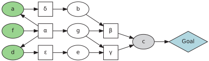
Unfortunately, even if the landmark graph Γ is sound and complete, using only nextLM makes the algorithm incomplete, as shown in the following counterexample. Let us consider the example in Figure 1 where circles are atoms, squares are actions, arrows mean precondition of an action or production of an atom and dashed arrows mean deletion of an atom. The initial state is {a, f, d} and the goal set is {c}. As we can see, g and c are landmarks, and g has to be reached before c. The first metanode will have the landmark g as goal. The subplanner gives the plan 〈α〉. The only generated metanode added to the open list is m = 〈{f, g}, h, {g}, c, 〈α〉〉. The associated problem Πm is unsolvable, as α deletes the preconditions of δ and ϵ which are mandatory actions that should be applied before α.
This led us to define new metanode generators, which, used in conjunction with nextLM, make the algorithm complete. These operators are based on landmark deletion from Γ, allowing for instance in the counterexample to try to reach the goal c without blindly focusing on g first.
Cut-parents Metanode Generation
These operators remove the ancestors of a non-root landmark.
Definition 11 (Cut-parents metanode generations). Let m = 〈s, h,A, l, ρ〉 be a metanode. If Πm has a solution ρ′ , then cutParent(m) = {〈s′ , h′ , A ∪ PΓ(l′ ), l′ , (ρ ◦ ρ′ )〉 | l′ ∈ ChΓ(l)} where s′ is the state obtained by applying ρ′ to s. If Πm has no solution, then cutParent(m) = ∅.
Definition 12 (Restart cut-parents metanode generation). restartCutParent(〈s, h,A, l, ρ〉) = {〈I, h′ ,A ∪ PΓ(l′ ), l′ , ∅〉 | l′ ∈ ChΓ(l)} where I is the initial state of the original planning problem.
The idea is that a total order constructed on the partial order defined by the landmark graph may be too restrictive, as in the counterexample. Using these two operators, some landmarks may be skipped by trying to reach deeper landmarks.
Delete Landmark Metanode Generation
Finally, we introduce the very generic landmark deletion operator: metanodes are generated as if the deleted landmark did not exist:
Definition 13 (Delete landmark metanode generation). deleteLM(〈s, h,A, l, ρ〉) = {〈s, h′ ,A ∪ {l}, l′ , ρ〉 | l′ ∈ roots(Γ \ (A ∪ {l}))}.
This operator discards a landmark, and causes the search to try to achieve remaining root landmarks. Applying this operator enough times on the first metanode (that has I as initial state) empties the landmark graph, eventually giving a metanode associated to the original planning problem. Also, the cut-parents operators can be seen as shortcuts for several delete landmark operators applications, guided by PΓ.
3.3 Algorithm
LMBFS (Algorithm 1) is a best-first search algorithm on metanodes of definition 7, with deferred heuristic evaluation [Richter and Helmert, 2009]: new nodes are inserted into the open list with the heuristic value of their parent.
Algorithm 1: LMBFS.
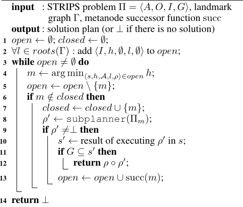
The algorithm is run on the problem Πg = 〈A ∪ {g}, O ∪ {ag}, I, {g}〉 where g is a dummy atom representing goal achievement, and ag is a dummy action whose precondition is G and add effect is {g}. g is a landmark whose achievement implies that a solution to Π has been found.
First, the metanodes associated to each root landmark of Γ are added to the open list. Then, at each iteration, the best metanode m (according to a heuristic detailed in section 3.4) is extracted from the open list, and a subplanner is run on the associated problem Πm. If the subplanner returns a plan, m is expanded by adding its successors to the open list. The algorithm iterates until the open list is empty or g is reached.
The function succ applied to the metanode m (Algorithm 1 line 13) computes the set obtained by an operator or the union set of several operators described in section 3.2. In our planner, we have implemeted two successor functions:
- succDel(m) = nextLM(m) ∪ deleteLM(m)
- succCut(m) = nextLM(m) ∪ cutParent(m) ∪ restartCutParent(m)
The operator nextLM is at the heart of our algorithm in order to focus on sequences of landmarks. However to ensure completeness, we have to use a combination of the other operators: as a net effect of applying these operators at each node expansion, the metanode m = 〈I, h′ , L \ {g}, g, ∅〉 corresponding to the global problem Πg will appear.
Theorem 1. The LMBFS algorithm using succCut or succDel as successor function is sound and complete if the subplanner is sound and complete.
Proof. (sketch) Soundness comes from: (1) the state in the first metanode is the initial state I of the problem, (2) all successor operators build plans that can be concatenated to form a solution of the global problem or search a new plan from I, and (3) if the final landmark g appears in a metanode, then achieving it solves the global problem goal. (2) is obtained by induction: if a metanode m = 〈s, h,A, l, ρ〉 is such that s is reachable by applying ρ from I, then by definition of nextLM and cutParent, s′ is the state obtained by applying ρ′ to s and so s′ is reachable by applying ρ ◦ ρ′ from I (using subplanner soundness). deleteLM modifies neither s nor ρ, so the recursive property is ensured. restartCutParent produces a metanode m = 〈I, h, A, l, ∅〉: a new search from I is started, giving a sound plan if the subplanner is sound.
Completeness comes from the fact that the operators restartCutParents (for the succCut successor function) and deleteLM (for the succDel successor function) are systematically used at each expansion of a metanode. So, the search graph contains a branch starting from the initial metanode consisting only of applications of restartCutParents or deleteLM, and both will have the effect to (1) keep I as associated state, (2) put all landmarks but g in the set of landmarks A, and (3) produce a final metanode whose associated landmark is g. From definition 9, opsΓ(g, L\{g}) = O∪{ag}: all actions of the original problem are used for solving this final metanode, which is the global problem, and so completeness of LMBFS derives from completeness of the subplanner.
Lazy Metanode Generation
The delete landmark metanode generation (section 3.2) can generate a considerable amount of metanodes for some instances, thus inducing a slow-down during the insertion of these metanodes in the open list. To overcome this issue, we generate metanodes with deleteLM only when the open list is empty. When a metanode is inserted in the closed list, it is also pushed into a secondary open list. When the main open list is empty, we simply pop a metanode m from the secondary open list, and generate its children using deleteLM(m). The heuristics for ordering metanodes in the secondary open list are the same as the ones used for the main open list.
3.4 Heuristics for Metanode Selection
In order to improve the algorithm effectiveness, the most promising metanode from the open list has to be selected. For doing so, a metanode generated by nextLM is always preferred over others, in order to focus search on reaching landmarks in sequence. Thus, the expansion of other (degraded) metanodes is delayed until we have no other choice, in the spirit that search can be focused using preferred operators [Richter and Helmert, 2009].
Three heuristic functions have been implemented. The first ones evaluate G from the starting state of the metanode, with the well-known heuristics hadd [Bonet and Geffner, 2001] and hff [Hoffmann and Nebel, 2001]. The last one, inspired by the landmark-counting heuristic of LAMA [Richter et al., 2008], uses the landmark graph Γ and counts the remaining landmarks to be reached. The metanode with the least number of remaining landmarks is chosen, enforcing a depth-first search in the graph. We will refer to this heuristic as hLleft .
Definition 14 (hLleft ). For a metanode m = 〈s, h,A, l, ρ〉 and an associated landmark graph Γ = (V, E), the heuristic hLleft is defined by hLleft (m) = |V \A|.
4 Experiments
4.1 Experimental Setup
We conducted a set of experiments on a selection of benchmarks from the 3 rd to the 7 th International Planning Competition (IPC) within a 10 minutes CPU time limit. The experiments were all run on an Intel X5670 processor running at 2.93Ghz with 24GB of RAM. In the next figures, each plot represents an IPC problem. Only results with the succDel operator are reported here, as it yielded better results than succCut. However, actually, nodes generated by nextLM are always preferred over nodes generated by these two operators, and we think that relevant heuristics for interleaving both kind of nodes might give a different picture.
Subplanner Embedded in LMBFS For subproblem resolution, we use YAHSP [Vidal, 2004; 2011] for two reasons.
Firstly, we do not want to use a subplanner that also uses landmarks internally (especially if non-negligible preprocessing time is required), as our objective is to evaluate a new use of landmarks without benefiting from them in any other way.
Secondly, because the successive subproblems solved during metanode expansion should be, and generally are, easy to solve with very few lookaheads computed in YAHSP. Moreover, directly embedded in the form of a C library, YAHSP does not require any preprocessing when faced with a new subproblem. It can thus generally answer very fast. It has also already been embedded with some success in another planner based on evolutionary algorithms [Biba¨ı et al., 2010] for solving different kinds of subproblem sequences.
SelectedDomains To come upwith a test suite, we ran preliminary tests in all STRIPS domains from the IPC. We selected some domains which YAHSP does not solve too easily (using few lookaheads), and also included some domains it solved easily to exhibit the possible slow-down required by the pre-computation of the landmark graph and the splitting into smaller instances of already easy solvable problems. Thus, we selected 14 domains 1 (390 problems), which we believe could represent a classic set of domains for the IPC.
4.2 Results
Landmark Graph Generation For most problems, the computation time of the landmark graph is low. It takes less than 0.1s for 86% of the instances, and less than 1s for 97% of the instances. Even if the computational time of the landmark graph on the initial state is acceptable, we consider it too long to be processed at each metanode during search. Recomputing landmarks could be more informative for search but, as LMBFS is designed for speed, we did not investigate such an option. Another reason is that adding new landmarks in the graph would break the current algorithm's completeness, which is based on emptying the initial landmark graph.
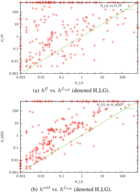
Efficiency of the Different Heuristics Figure 2(a) shows a comparison of the runtime of LMBFS with hLleft (x-axis) and hff (y-axis). As we can see, most of the plots are above y = x, meaning most instances have been solved faster using hLleft . Figure 2(b) shows a comparison between hLleft (x-axis) and hadd (y-axis). The results are again in favor of hLleft which outperforms hadd in most of the problems. Table 1 summarizes the runs performed with LMBFS using several heuristics. It shows that LMBFS with the hLleft heuristic outperforms the two other (with hadd or hff ).
| Heuristic | solved < 1s | solved < 10s | solved |
|---|---|---|---|
| hadd | 45.64% | 63.85% | 75.13% |
| hff | 34.62% | 45.38% | 57.95% |
| hLleft | 74.36% | 85.90% | 92.31% |
Lazy Metanode Generation Table 2 compares the speedup obtained by using the lazy metanode generation described in section 3.3. We can see that there is a strictly positive speed-up for 51.03% of the problems, and a speed-up superior to 2 for 23.74% of them. Even if there is a noticeable slow-down for 4.36% of the problems (heuristically equivalent nodes may be ordered differently in the main and secondary open lists due to implementation details), it still is a nice improvement for the overall test suite.
1 ipc3-driverlog, ipc3-freecell, ipc3-satellite, ipc4-pipesworld - tankage, ipc4-psr small, ipc[56]-openstacks, ipc5-pathways, ipc[67]-transport, ipc[67]-scanalyzer, ipc7-barman, ipc7-floortile
| Instances where the speed-up/slow-down is | ||||
|---|---|---|---|---|
| Average | > 1 | > 1.05 | > 2 | |
| Speed-up | 8.11 | 51.03% | 36.41% | 22.74% |
| Slow-down | 2.24 | 14.10% | 4.36% | 1.81% |
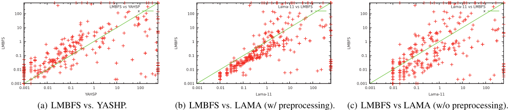
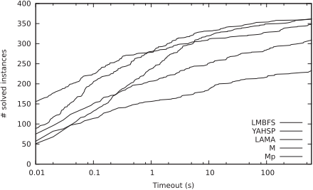
LMBFS versus sub-planner (YAHSP) Table 3 summarizes the coverage of runs performed with LMBFS using the hLleft heuristic in comparison with YAHSP and some stateof-the-art planners, also shown as a curve in function of the timeout in Figure 4. The comparison between LMBFS and YAHSP is also depicted in Figure 3(a). It shows that many problems are solved within 1s and most of the problems quickly solved by YAHSP (under 0.1s) are solved by LMBFS nearly as fast. On harder instances we can also see that LMBFS shows its benefits in terms of running time. Finally the total number of solved instances is slightly in favor of LMBFS.
A major drawback that has been pointed out for the DSC algorithm and the SteLLa planner is the length of computed plans which can be significantly higher. Compared to the plans computed by YAHSP, the average plan length computed by LMBFS is 8% shorter. In 43% instances LMBFS computes strictly shorter plan than YAHSP and in 19% instances the plans are strictly longer.
LMBFS versus State-of-the-Art Planners Table 3 and Figure 4 compare LMBFS to the LAMA-11 planner (based on landmark analysis but in a different way), as well as to the SAT-based planners M and Mp [Rintanen, 2012].
Figures 3(b) and 3(c) are scatter plots comparing the runtimes of LMBFS versus LAMA-11. Figure 3(b) shows runtimes including preprocessing within the 10 minutes timeout, and Figure 3(c) without taking into account the preprocessing time, as LAMA-11 can spend a lot of time during this stage.
These evaluations show that on our selection of domains, LMBFS is competitive with the state-of-the-art. It clearly outperforms M, Mp and YAHSP (for problems that require at least 1 second). It also outperforms LAMA-11, although the overall performance for a 10 minutes timeout depends on whether or not the preprocessing time is included.
5 Conclusion and FutureWorks
This paper presents several contributions towards a new landmark-based planning algorithm. First, we propose a sound framework for a (meta)search based on the order of landmarks, given a landmark graph. We formalize the link between so-called metanodes and subproblems of the original planning problem, including restrictions on the allowed actions themselves. We give several operators that allow to explore different orders for using landmarks as subgoals, including skipping some. We also propose a first approach for evaluating heuristic values of such metanodes, or equivalently giving priorities to subproblems. We put everything together in a (deferred) best-first search algorithm, leading to a complete algorithm. Last but not least, we implemented it and give some promising results.
| Planner | solved < 1s | solved < 10s | solved |
|---|---|---|---|
| with preprocessing time | |||
| LMBFS | 71.79% | 84.87% | 92.31% |
| YAHSP | 71.28% | 79.74% | 88.97% |
| LAMA-11 | 60.51% | 81.79% | 92.05% |
| M | 40.00% | 47.44% | 58.72% |
| Mp | 52.82% | 64.36% | 78.46% |
| without preprocessing time | |||
| LMBFS | 74.36% | 85.90% | 92.31% |
| LAMA-11 | 69.74% | 82.82% | 92.56% |
From now on, several leads will be followed.
A key point for performance is the heuristic evaluation of metanodes, linked to the operators used for generation. For instance, nodes generated with nextLM are always expanded before other metanodes, which is not necessarily the best solution. A first lead to obtain a better heuristic would be to also take into account the landmark subgoal but preliminary experiments showed us that this will not be straightforward.
Another point is the operators used. While deleteLM is very general, cutParent can be seen as a special case (a shortcut for a given sequence of deleteLM, or said differently, a lookahead in the landmark graph itself), and other special cases may be very useful.
Another future work consists in modifying the LMBFS algorithm to make it distributed for being executed on new parallel architectures. A first scheme based on ideas from HDA* [Kishimoto et al., 2009] is proposed in [Vernhes et al., 2013].
@inproceedings{ijcai2013p353,
  title     = {Problem Splitting Using Heuristic Search in Landmark Orderings},
  author    = {Vernhes, Simon and Infantes, Guillaume and Vidal, Vincent},
  booktitle = {Proceedings of the Twenty-Third International Joint Conference on
               Artificial Intelligence, {IJCAI-13}},
  publisher = {AAAI Press / International Joint Conferences on Artificial Intelligence},
  editor    = {Francesca Rossi},
  pages     = {2401--2406},
  year      = {2013},
  month     = {8},
  url       = {https://ijcai.org/proceedings/2013/353},
}
TY - CPAPER TI - Problem Splitting Using Heuristic Search in Landmark Orderings AU - Vernhes, Simon AU - Infantes, Guillaume AU - Vidal, Vincent T2 - Proceedings of the Twenty-Third International Joint Conference on Artificial Intelligence, IJCAI-13 PB - AAAI Press / International Joint Conferences on Artificial Intelligence PY - 2013 SP - 2401 EP - 2406 UR - https://ijcai.org/proceedings/2013/353 ER -Copied
Machine-readable versions of this paper, for tools and AI agents:





