
Revenue Maximization via Hiding Item Attributes
Proceedings of the Twenty-Third International Joint Conference on Artificial Intelligence. Pages 157-162.
© 2013 International Joint Conferences on Artificial Intelligence
Abstract
We study probabilistic single-item second-price auctions where the item is characterized by a set of attributes. The auctioneer knows the actual instantiation of all the attributes, but he may choose to reveal only a subset of these attributes to the bidders. Our model is an abstraction of the following Ad auction scenario. The website (auctioneer) knows the demographic information of its impressions, and this information is in terms of a list of attributes (e.g., age, gender, country of location). The website may hide certain attributes from its advertisers (bidders) in order to create thicker market, which may lead to higher revenue. We study how to hide attributes in an optimal way. We show that it is NP-hard to compute the optimal attribute hiding scheme. We then derive a polynomial-time solvable upper bound on the optimal revenue. Finally, we propose two heuristic-based attribute hiding schemes. Experiments show that revenue achieved by these schemes is close to the upper bound.
- [Avery and Hendershott, 2000] Christopher Avery and Ter- rence Hendershott. Bundling and optimal auctions of mul- tiple products. Review of Economic Studies, 67:483-497, 2000.
- [Bro Miltersen and Sheffet, 2012] Peter Bro Miltersen and Or Sheffet. Send mixed signals: earn more, work less. In Proceedings of the ACM Conference on Electronic Com- merce (EC), Valencia, Spain, 2012.
- [Chakraborty, 1999] Indranil Chakraborty. Bundling deci- sions for selling multiple objects. Economic Theory, 13(3):723-733, 1999.
- [Emek et al., 2012] Yuval Emek, Michal Feldman, Iftah Gamzu, Renato Paes Leme, and Moshe Tennenholtz. Sig- naling schemes for revenue maximization. In Proceedings of the ACM Conference on Electronic Commerce (EC), Va- lencia, Spain, 2012.
- [Even-Dar et al., 2007] Eyal Even-Dar, Michael Kearns, and Jennifer Wortman. Sponsored search with contexts. In Workshop on Internet and Network Economics (WINE), San Diego, CA, USA, 2007.
- [Ghosh et al., 2007] Arpita Ghosh, Hamid Nazerzadeh, and Mukund Sundararajan. Computing optimal bundles for sponsored search. In Workshop on Internet and Network Economics (WINE), San Diego, CA, USA, 2007.
- [Leyton-Brown et al., 2000] Kevin Leyton-Brown, Mark Pearson, and Yoav Shoham. Towards a universal test suite for combinatorial auction algorithms. In Proceedings of the ACM Conference on Electronic Commerce (EC), pages 66-76, Minneapolis, MN, USA, 2000.
- [Palfrey, 1983] Thomas R Palfrey. Bundling decisions by a multiproduct monopolist with incomplete information. Econometrica, 51(2):463-83, March 1983.
- [Schaefer, 1978] Thomas J. Schaefer. The complexity of sat- isfiability problems. In Proceedings of the Annual Sympo- sium on Theory of Computing (STOC), San Diego, Cali- fornia, USA, 1978.
References were extracted automatically from the PDF and may contain errors.
Full text extracted automatically from the PDF; figures, tables and equations may differ. The PDF is the version of record.
1 Introduction
One advantage of Internet advertising is that it offers advertisers the ability to target customers based on various traits such as demographics. [Even-Dar et al., 2007] showed that, for sponsored search of a given keyword, instead of running a single auction for the keyword, we can split the whole auction into many separate auctions based on visitors/impressions' contexts (e.g., demographics). For example, if we know and only know the visitors' locations, then each location defines a context. In this example scenario, splitting based on context means separate auction for each location. Splitting based on context increases the advertisers' welfare. The explanation is simple: after splitting, advertisers can tailor their bids to the context. As a result, advertisers generally only win (impressions from) visitors that they aim to target. On the other hand, splitting may reduce the revenue received by the auctioneer (publisher, e.g., website) due to the thin market
∗This work was supported by Microsoft Research through its PhD Scholarship Programme.
Argyrios Deligkas
Department of Computer Science University of Liverpool, UK A.Deligkas@liverpool.ac.uk
problem: there may be few competitors for some contexts. Actually, if for every context, there is only one advertiser interested in it, then the total revenue is 0 under the standard second-price auction.
[Ghosh et al., 2007] observed that having a single auction for all contexts and having separate auction for each context are not the only two options. There are other ways to split based on context, and it may lead to much higher revenue. The idea explored in [Ghosh et al., 2007] is to cluster the contexts into bundles, and run separate auction for each bundle. For example, suppose there are three different contexts: Beijing, Chicago, and London (assuming the only contextual information is the location and visitors are only from these three cities). We can have one auction for the bundle Beijing and Chicago (and a second auction for London only). The interpretation (due to [Emek et al., 2012]) is that if a visitor is from Beijing or Chicago, then the auctioneer informs the advertisers that the impression is from one of these two cities, but not exactly which. When this happens, both advertisers targeting Beijing and advertisers targeting Chicago will compete in the auction. Their bids depend on how much they value impressions from Beijing and Chicago, respectively. Their bids also depend on the conditional probability that the impression is from Beijing (or Chicago) given that the impression is from one of these two cities.
To put it more formally, [Ghosh et al., 2007] studied probabilistic single-item second-price auctions (again, interpretation due to [Emek et al., 2012]). In such an auction, there is only one item for sale under a second-price auction, but the item has different possible instantiations. The auctioneer knows the actual instantiation but the bidders do not. The auctioneer may choose to hide certain information from the bidders if this increases the revenue. The probabilistic single-item second-price auction model is an abstraction of the following Ad auction scenario. We have a website that sells one advertisement slot. That is, there is only one item - the only advertisement slot, but the item takes many possible instantiations, due to the fact that visitors/impressions have different demographic profiles. The auctioneer knows every visitor's demographic profile, and he may hide certain information from the advertisers. As mentioned above, [Ghosh et al., 2007] considered hiding information by clustering: the auctioneer tells the bidders that the actual instantiation is among several instantiations. [Emek et al., 2012;
Bro Miltersen and Sheffet, 2012] studied the exact same model and went one step further. These two papers studied hiding information by signaling: the auctioneer sends out different signals, and the bidders infer the probability distribution of the actual instantiation, based on the signal received. It is easy to see that signaling is more general than clustering. Interestingly, for full information settings (settings where the auctioneer knows the bidders' exact valuations), [Ghosh et al., 2007] showed that it is NPhard to compute the optimal clustering scheme (optimal in terms of revenue). On the other hand, [Emek et al., 2012; Bro Miltersen and Sheffet, 2012] both independently showed that, under the same full information assumption, it takes only polynomial time to solve for the optimal signaling scheme. This is mostly due to the fact that instantiations are treated as divisible goods under signaling schemes,
In this paper, we continue the study of revenue-maximizing probabilistic single-item second-price auctions. We observe that in practice, Ad impressions are categorized based on multiple attributes. Given this, we argue that the most natural way to hide information is by hiding attributes. For example, let there be three attributes, each with two possible values:
- Age: Teenager, Adult
- Gender: Male, Female
- Location: US, Non-US
Together there are 23 possible instantiations. Under the clustering scheme studied in [Ghosh et al., 2007], the website is allowed to hide information by bundling any subset of instantiations. However, not all bundles are natural. For example, consider the bundle {(Teenager, Male, US), (Adult, Female, Non-US)}. By creating this bundle, the website basically may tell the advertisers that a visitor is either a teenage US male or an adult Non-US female. This does not appear natural. The signaling scheme studied in [Emek et al., 2012; Bro Miltersen and Sheffet, 2012] is even more general than clustering, so it may also lead to unnatural bundles.
On the other hand, attribute hiding always leads to natural bundles. For example, the website may hide the location attribute. That is, if the actual instantiation is (Teenager, Male, US), then the website may inform the advertisers that the visitor is a teenage male. By hiding the location attribute, we essentially created a bundle (Teenager, Male, ?), which consists of both (Teenager, Male, US) and (Teenager, Male, Non-US).
Based on the above example, it is easy to see that attribute hiding is clustering with a particular structure. It should be noted that this relationship between attribute hiding and clustering does not mean previous results on clustering apply to our model. For example, one of the two main results from [Ghosh et al., 2007] is a constructed clustering scheme that guarantees one half of the optimal revenue (and one half of the optimal social welfare). The construction does not apply to our model since it generally leads to unnatural bundles.
In this paper, we first show that it is NP-hard to compute the optimal attribute hiding scheme. 1 We then derive a polynomial-time solvable upper bound on the optimal revenue. Finally, we propose two heuristic-based attribute hiding schemes. Experiments show that revenue achieved by these schemes is close to the upper bound.
1 We mentioned earlier that [Ghosh et al., 2007] proved a similar result. The authors showed that it is NP-hard to solve for the optimal clustering scheme. It should be noted that our NP-hardness result is
Besides the aforementioned related work in the computer science literature, bundling has also been well-studied in the economics literature. [Palfrey, 1983] observed that for small numbers of bidders, a revenue-maximizing auctioneer may choose to bundle the items, and this makes bidders universally worse-off. On the other hand, for large numbers of bidders, the auctioneer may choose to unbundle the items, and this hurts the high-demand bidders while benefiting the low-demand bidders. [Chakraborty, 1999] quantitatively analyzed the bundling behavior of the auctioneer. The result is that under a Vickrey auction, for each pair of objects, there is a unique critical number. If there are fewer bidders than this number, the seller chooses to bundle the items, and vice versa. [Avery and Hendershott, 2000] studied more sophisticated bundling policy, including bundling with discounts and probabilistic bundling (the probability of bundling occurring depends on the bids).
2 Model Description
There is a single item for sale characterized by k attributes (attribute 1 to k). Attribute i has Ci possible values, ranging from 0 to Ci - 1. Let m be the total number of possible instantiations. That is, m = ∏i Ci. In this paper, when we mention polynomial time or NP-hardness, we mean in terms of m.
An instantiation whose i-th attribute equals ai is written as
The space of all possible instantiations Ω is
Definition 1. A natural bundle b is an element from the following set of all natural bundles (denoted by B):
Natural bundles are bundles of instantiations resulting from hiding attributes. An attribute of a natural bundle either takes a specific value, or is represented by a question mark, which means that this attribute is hidden. For example, let k = 5, given the instantiation (a1, a2, a3, a4, a5), if we hide attributes 1 and 3, then it results in the natural bundle (?, a2, ?, a4, a5). This bundle has size C1C3. As another example, every instantiation itself corresponds to a natural bundle of size 1 (no attribute hidden). An instantiation ω belongs to a natural bundle b if and only if for every attribute, either ω and b share the same attribute value, or the attribute is hidden for b. Unlike the total number of arbitrary bundles, which equals 2m, the total number of natural bundles is polynomial in m, as shown below:
not implied by this earlier result, which relied on reduction involving unnatural bundles. Actually, our requirement on bundles being natural greatly adds to the difficulty of the reduction, and our proof is based on completely new techniques.
The probabilities' of different instantiations are based on a publicly known distribution ∆(Ω). To simplify the presentation, when discussing bidders' valuations, we factor in the probabilities. For example, if bidder i values ω at 5 when ω is the actual instantiation, and ω happens with probability 0.1, then we say bidder i's valuation for ω is 0.5.
Let n be the number of bidders. Let vi(ω) be bidder i's (expected) valuation for instantiation ω. Following [Ghosh et al., 2007; Emek et al., 2012; Bro Miltersen and Sheffet, 2012] 2 , we assume full information: the auctioneer knows the bidders' true valuations. Again, following previous models, we only consider bidders with additive valuations. That is, bidder i's valuation for bundle b, denoted by vi(b), equals ∑ω∈b vi(ω). Following previous models, the auction is the Vickrey auction. We use S(b) to denote the revenue for selling b as a bundle. S(b) is the second highest value in {vi(b)|1 ≤ i ≤ n}.
Definition 2. An attribute hiding scheme is a way to cluster the instantiations into natural bundles. An attribute hiding scheme is characterized by a set of bundles {b1, b2, . . . , bt}, satisfying
- All bundles are natural: bi ∈ B for 1 ≤ i ≤ t
- The bundles are disjoint 3 : for every pair of bi and bj, there exists an attribute, so that for this attribute, bi and bj take different values (neither is ?).
Under the attribute hiding scheme {b1, b2, . . . , bt}, instantiations covered by bi will have their attributes hidden to match bi. Essentially, instantiations in bi are sold in a bundle. Instantiations not covered by any bi are sold without hiding attributes (sold separately as natural bundles of size 1).
Under attribute hiding scheme {b1, b2, . . . , bt}, the revenue of the auctioneer equals
We introduce another function r. For b ∈ B, r(b) represents the extra revenue obtained by selling b as a bundle, rather than selling instantiations in b separately. We have
The revenue of the auctioneer can then be rewritten as
The second term of the above expression does not depend on the specific scheme. Therefore, the problem of designing optimal attribute hiding scheme is equivalent to the problem of searching for a set of disjoint natural bundles {b1, b2, . . . , bt}, so that ∑1≤i≤t r(bi) is maximized.
2 Besides the full information setting, [Emek et al., 2012] also discussed the more general Bayesian setting.
3 If under an attribute hiding scheme, two different natural bundles share one common instantiation, then for this instantiation, it is not clear which attributes we should hide.
3 Hardness Result
Previously, [Ghosh et al., 2007] showed that it is NP-hard to compute the optimal clustering scheme. The proof was by reduction from 3-partition. In this section, we prove a similar result. We show that it is also NP-hard to compute the optimal attribute hiding scheme. Our proof is by reduction from monotone one-in-three 3SAT [Schaefer, 1978]. Monotone one-in-three 3SAT is a variant of 3SAT. Monotone means that the literals are just variables, never negations. One-in-three means that the determination problem is to see whether there is an assignment so that for each clause, exactly one literal is true.
Theorem 1. It is NP-hard to compute the optimal attribute hiding scheme.
Proof. Let us consider the following monotone one-in-three 3SAT instance with D clauses:
There are 3D literals, and they are from a list of E variables (x1 to xE, f's range is between 1 and E). According to [Schaefer, 1978], it is NP-complete to determine whether there exists an assignment of the xi, so that the 3SAT instance is true, and for each clause, there is exactly one true literal.
We will construct a probabilistic single-item auction scenario with m possible instantiations and n bidders. Both m and n are polynomial in E. We will show that for the constructed scenario, if we are able to solve for the optimal attribute hiding scheme in polynomial time (in m), then we are able to determine the above 3SAT instance in polynomial time (in E). This implies that it is NP-hard to compute the optimal attribute hiding scheme.
Our construction is as follows. Let the number of attributes k be ⌈log2(D)⌉ + ⌈log2(E)⌉ + 11. All attributes are binary. The total number of instantiations m is polynomial in E as shown below.
Our proof relies on the following seven families of natural bundles (Family 1 to 7):
In the above, e is the binary representation of integer e (1 ≤ e ≤ E). The representation's width is ⌈log2(E)⌉. Similarly, d is the binary representation of integer d (1 ≤ d ≤ D). The representation's width is ⌈log2(D)⌉. Finally, ? is ? repeated ⌈log2(E)⌉ times (Family 5, 6, and 7) or ⌈log2(D)⌉ times (Family 4).
We recall that the problem of designing optimal attribute hiding scheme is equivalent to the search of disjoint natural bundles {b1, b2, . . . , bt}, so that ∑1≤i≤t r(bi) is maximized. Given a natural bundle b, r(b) depends on the bidders' valuations. We will construct a set of bidders, so that for any natural bundle b, r(b) = 0 by default. The exceptions are:
- For i = 1, 2, 3, we use bi (e, d) to represent the natural bundle characterized by e and d in Family i. r(bi (e, d)) = 1 if and only if, in the 3SAT instance, variable e appears in the i-th position of clause d.
- We use b4 (e) to represent the natural bundle characterized by e in Family 4. Let N(e) be the number of times variable e appears in the 3SAT instance. It is without loss of generality to assume N(e) ≤ D (no literal appears twice in a clause). Let r(b4 (e)) = N(e)(1 - ϵ). Here, ϵ is a constant that is less than 1D . The idea is to make sure that N(e)(1 - ϵ) > N(e) - 1.
- We use b5 (d) to represent the natural bundle characterized by d in Family 5. r(b5 (d)) = 3.
- We use b6 (d) to represent the natural bundle characterized by d in Family 6. r(b6 (d)) = 3.
- We use b7 (d) to represent the natural bundle characterized by d in Family 7. r(b7 (d)) = 3.
For now, we simply assume that it is possible to construct a polynomial number of bidders, so that the values of r(b) for different b are indeed as described above. We will provide the specific construction toward the end.
Let O be an optimal attribute hiding scheme corresponding to the above construction. If r(b) = 0, then it is without loss of generality to assume b /∈ O. Therefore, we can ignore bundles not in the above seven families. Some bundles from Family 1 to 3 can also be ignored for the same reason. For presentation purposes, we call the remaining bundles helpful bundles. A bundle b is helpful if and only if r(b) > 0.
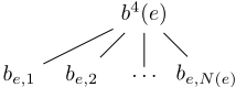
Let us consider a fixed variable e (1 ≤ e ≤ E). e appears N(e) times in the 3SAT instance, so there are exactly N(e) pairs of d (1 ≤ d ≤ D) and i (1 ≤ i ≤ 3), so that bi (e, d) is helpful. We use be,1, be,2, . . . , be,N(e) to denote these N(e) helpful bundles. They are the only helpful bundles that intersect b4 (e). If some of these bundles are not in O, then none of them is in O. The reason is that r(b4 (e)) = N(e)(1 - ϵ) > N(e) - 1, so it is better off to add b4 (e) into O (and push out be,1 to be,N(e) if they are in O). In summary, for e from 1 to E, we must have one of the following two:
- be,1, be,2, . . . , be,N(e) are all in O. b4 (e) is not in O.
- None of be,1, be,2, . . . , be,N(e) is in O. b4 (e) is in O.
Let T be the set of e values where be,1, be,2, . . . , be,N(e) are all in O. Let F be the set of e values where none of be,1, be,2, . . . , be,N(e) is in O. We use O1234 to denote the set of helpful bundles in O that belong to Family 1 to 4. We have
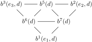
Let us then consider a fixed variable d (1 ≤ d ≤ D). b5 (d), b6 (d), and b7 (d) pair-wise intersect. Therefore, in O, at most one of them can appear. Actually, exact one of them appears. If none of them appears in O, then we can add b5 (d) into O, which results in higher revenue. Let e2 and e3 be the second and third variables in clause d of the 3SAT instance. The only helpful bundles b5 (d) intersects with are b2 (e2, d) and b3 (e3, d). By removing these two from O (if they are in O to start with) and adding b5 (d) into O, the revenue increases. Therefore, for any d from 1 to D, O contains exactly one of {b5 (d), b6 (d), b7 (d)}. We use O567 to denote the set of helpful bundles in O that belong to Family 5 to 7. We have
Among helpful bundles characterized by d from Family 1 to 3, the only helpful bundle that can coexist with b5 (d) is b1 (e1, d), where e1 is the first variable in clause d of the 3SAT instance. Similarly, among helpful bundles characterized by d from Family 1 to 3, the only helpful bundle that can coexist with b6 (d) is b2 (e2, d), where e2 is the second variable in clause d of the 3SAT instance. Finally, among helpful bundles characterized by d from Family 1 to 3, the only helpful bundle that can coexist with b7 (d) is b3 (e3, d), where e3 is the third variable in clause d of the 3SAT instance. The relationship is illustrated by Figure 2.
For every d, no matter which of {b5 (d), b6 (d), b7 (d)} appears in O, among helpful bundles characterized by d from Family 1 to 3, there is at most one that can be in O. Therefore, the total number of helpful bundles from Family 1 to 3 in O is at most D.
If we are able to compute the optimal attribute hiding scheme in polynomial time, then we are also able to determine in polynomial time whether ∑b∈O r(b) is equal to the upper bound 6D - 2Dϵ. If they are equal, then we have a satisfactory assignment of the 3SAT instance. For variable e, be,1 to be,N(e) determine whether e is true or not. If they are all in O, then e is set to be true. Otherwise (if none of them is in O), e is set to be false. When the upper bound is reached, ∑e∈T N(e) = D, which implies that under the above assignment, there are exactly D true literals. Next, we show that two true literals cannot appear in the same clause. That is, there is exactly one true literal for each clause under the assignment, and all clauses are satisfied (there are D true clauses). Given d, let the variables in clause d be e1, e2, e3. b1 (e1, d), b2 (e2, d), and b3 (e3, d) are all helpful bundles. We proved that among helpful bundles characterized by d from Family 1 to 3, there is at most one that can be in O. Therefore, only one of b1 (e1, d), b2 (e2, d), b3 (e3, d) can be in O. That is, only one of e1, e2, e3 is set to be true.
The other direction can be shown similarly. If there is a satisfactory assignment of the 3SAT instance, then ∑b∈O r(b) should match the upper bound 6D - 2Dϵ.
In conclusion, for the constructed auction setting, it is NPhard to determine whether the optimal revenue ∑b∈O r(b) + ∑ω∈Ω S(ω) reaches 6D - 2Dϵ + ∑ω∈Ω S(ω).
Finally, we still need to show that it is possible to construct a polynomial number of bidders, so that the values of r(b) are exactly as described above. Due to space constraint, we present the construction and omit the proof.
- We construct two bidders who both value every instantiation equally, and the valuation for every instantiation is L (L > max{D, 3}).
- For every helpful bundle b, we construct two new bidders. By default, both bidders value all instantiations in b at L and value all instantiations outside of b at 0. The exceptions are that one bidder values instantiation b|0? at r(b) + L and the other bidder values instantiation b|1? at r(b) + L. Here, b|y? is the instantiation resulting from replacing all ? in b by y.
4 Tree-Structured Attribute Hiding Schemes
In this section, we study a special family of attribute hiding schemes, which we call the tree-structured schemes.
Let b be a non-unit natural bundle (bundle of size greater than 1). For b, at least one attribute is hidden. Let x be one of the hidden attributes of b. We can split b into Cx disjoint natural bundles by revealing attribute x. The resulting bundles are b|0x , b|1x , . . . , b|Cx-1 x . b|ix represents the natural bundle obtained by replacing the x-th attribute of b by i. If b belongs to an attribute hiding scheme O, then after splitting b, the new scheme becomes
It is easy to see that the new scheme is still feasible (the bundles remain disjoint).
Tree-structured attribute hiding schemes are results of recursive splitting (revealing attribute) starting from {(?, ?, . . . , ?)}. At every step, we either terminate and keep the current scheme, or pick a non-unit bundle from the current scheme, and split (reveal) one of its attributes.
Definition 3. An attribute hiding scheme O is tree-structured if and only if it satisfies one of the following:
- O = {(?, ?, . . . , ?)}: the scheme is simply hiding all attributes and selling all instantiations in a single bundle.
- There exists a tree-structured attribute hiding scheme O′ . There exists a bundle b ∈ O′ whose x-th attribute is hidden. After splitting b by revealing attribute x, the resulting scheme is equivalent to O. 4
Let us consider an example with three binary attributes. {(?, ?, ?)} is, by definition, a tree-structured attribute hiding scheme. Starting from {(?, ?, ?)}, if we pick (?, ?, ?) and reveal its second attribute, then we get
The leaves {(?, 0, ?), (?, 1, ?)} characterize a new treestructured attribute hiding scheme. If we further split the first bundle (?, 0, ?) based on its third attribute, then we get
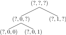
Again, the leaves {(?, 0, 0), (?, 0, 1), (?, 1, ?)} characterize a new tree-structured attribute hiding scheme.
Proposition 1. If there are at most two attributes, then all attribute hiding schemes are tree-structured. 5
Proposition 2. If there are at least three attributes, then there exist attribute hiding schemes that are not tree-structured.
As we mentioned earlier, tree-structured attribute hiding schemes are results of recursive splitting starting from the bundle of all instantiations. At every step, we either terminate or split a non-unit bundle in some way. For every natural bundle b, let t(b) be the optimal revenue for selling instantiations in b, as a result of making optimal recursive splitting decisions on b. t((?, ?, . . . , ?)) is then the optimal revenue of tree-structured attribute hiding schemes. Given a bundle, we either sell it as a whole, or split it in some way as a first step. Let h(b) be the set of hidden attributes of b. We have
If b has size 1, then h(b) = ∅. That is, for unit bundles, t(b) = S(b). Given the values of t(b) for all b with
4 Two schemes are equivalent if they share the same set of nonunit bundles.
5 This proposition implies that if there are at most two attributes (m can still be large), then we can compute the optimal attribute hiding scheme in polynomial time, because it must be tree-structured.
|h(b)| = y, we can then easily compute the values of t(b) for all b with |h(b)| = y+1. The total number of natural bundles |B| is polynomial in m. For every b, t(b) is the maximum of at most k + 1 values, which is at most log2m+ 1. Therefore, the optimal revenue t((?, ?, . . . , ?)) can be computed in polynomial time. The corresponding optimal scheme can be obtained along the way.
5 Upper Bound andWeightedMatching
Our objective is to find a set of disjoint natural bundles, denoted by O, which maximizes ∑b∈O r(b). We can model it as an integer program. We introduce |B| binary variables. For b ∈ B, let zb be a binary variable. If zb = 1, then it means b ∈ O. The number of binary variables |B| is polynomial in m. The objective is to maximize ∑b∈B zbr(b). The constraints are that bundles in O are disjoint. That is, for b1, b2 ∈ B, if b1 and b2 intersect, zb1 + zb2 ≤ 1. The number of constraints is at most |B|2 , which is polynomial in m. In summary, the optimal revenue can be computed based on an integer program with polynomial numbers of variables and constraints. One upper bound can then be computed in polynomial time if we consider the linear relaxation (replacing binary variables by non-integer variables).
Some preprocessing can vastly reduce the number of variables in the above program. We first observe that, by definition, r(b) = 0 for all b with size 1. That is, we can safely set zb = 0 for all b with size 1. We then observe that, for any natural bundle b with size greater than 1, if the following expression is true, then it means that instead of selling b as a single bundle, we can achieve higher revenue by recursively splitting it, in which case we can safely set zb = 0.
In Section 6, our simulation shows that when computing the upper bound, the above observations indeed vastly reduce the number of variables in the linear program. For example, for settings with 10 binary attributes and 10 bidders, originally, there are as many as (2 + 1)10 = 59049 variables. After preprocessing, there are only 220.28 variables on average over repeated simulations.
We then discuss another heuristic for generating attribute hiding schemes with high revenue. This heuristic only applies to settings where all attributes are binary. If all attributes are binary, then a natural bundle with only one attribute hidden contains exactly two instantiations. The heuristic is based on maximum weighted matching. We view all instantiations as vertices. If two instantiations can be merged into a natural bundle b, and r(b) > 0, then we create an edge with weight r(b) between them. Maximum weighted matching can be solved in polynomial time. The matching result characterizes the optimal attribute hiding scheme under the additional constraint that at most one attribute is hidden. 6
6 In Section 6, our simulation shows that there are generally very few natural bundles with at least two hidden attributes, and cannot be recursively split to achieve higher revenue. That is, the optimal scheme generally contains very few bundles with two or more hidden attributes. This somewhat justifies the heuristic requirement that at most one attribute is hidden.
6 Experiments
In this section, we evaluate the performances of the proposed heuristic-based attribute hiding schemes. For different values of k, ¯ C, and n, we construct problem instances with k attributes, each attribute taking ¯ C possible values, and n bidders. The total number of possible instantiations is then ¯ C k . For each instantiation, bidders' valuations are drawn independently from U(0, 1). 7 For every setup, we repeat 100 times and report the averages.
| Setup | Tree | Match | UB | #Opt | #Var | HM |
|---|---|---|---|---|---|---|
| k = n = 3 ¯ C = 2 | 13.33 | 11.58 | 15.42 | 47 | 5.82 | 1.08 |
| k = n = 5 ¯ C = 2 | 3.953 | 3.810 | 4.354 | 35 | 15.8 | 1.54 |
| k = n = 10 ¯ C = 2 | 0.836 | 0.927 | 0.950 | 0 | 220.28 | 4.76 |
| k = n = 3 ¯ C = 3 | 9.251 | NA | 10.58 | 25 | 13.28 | 0.96 |
| k = n = 5 ¯ C = 3 | 1.767 | NA | 1.976 | 0 | 45.39 | 0.3 |
| k = n = 8 ¯ C = 3 | 0.296 | NA | 0.361 | 0 | 326.18 | 0.01 |
The table fields are described below:
- Tree, Match, UB: Comparing to selling all instantiations separately, the extra revenue in terms of percentage. Tree is short for optimal tree-structured scheme. Match is short for optimal scheme based on maximum weighted matching (only applies to ¯ C = 2). UB is short for upper bound on the optimal revenue.
- #Opt: Among 100 repeated simulations, how many times one of the heuristic-based schemes reaches the upper bound (therefore guarantees optimality 8 ).
- #Var: How many variables are in the linear program for computing upper bound.
- HM: How many natural bundles with at least two hidden attributes cannot be split to achieve higher revenue.
7 Future Research
Given the fact that it is NP-hard to compute the optimal attribute hiding scheme, one direction of future research is to study whether there are heuristic-based attribute hiding schemes that guarantee a constant fraction of the optimal revenue. A similar direction is to see how much revenue we lose by not allowing unnatural bundles.
7 We also experimented with the CATS test suite [Leyton-Brown et al., 2000]. Our model assumes additive valuations, so we need to contrive a way to interpret the bids produced by CATS as additive bids. One example way is to interpret each bid as an individual additive bidder. Given a bid, if an item belongs to it, then we assume that the corresponding bidder's valuation for the item is equal to the value of the bid, and otherwise 0. Under the above assumption, for 8 goods (3 binary attributes), 3 bidders (ignore all bids after the first 3), and the arbitrary distribution, over 100 instances, the optimal tree-based scheme increases the revenue by 6.38 percent (compared to not bundling), and it is close to the upper bound 7.76 percent.
8 Even if the heuristic-based schemes do not reach the upper bound, they may still possibly be optimal.
@inproceedings{ijcai2013p33,
  title     = {Revenue Maximization via Hiding Item Attributes},
  author    = {Guo, Mingyu and Deligkas, Argyrios},
  booktitle = {Proceedings of the Twenty-Third International Joint Conference on
               Artificial Intelligence, {IJCAI-13}},
  publisher = {AAAI Press / International Joint Conferences on Artificial Intelligence},
  editor    = {Francesca Rossi},
  pages     = {157--162},
  year      = {2013},
  month     = {8},
  url       = {https://ijcai.org/proceedings/2013/33},
}
TY - CPAPER TI - Revenue Maximization via Hiding Item Attributes AU - Guo, Mingyu AU - Deligkas, Argyrios T2 - Proceedings of the Twenty-Third International Joint Conference on Artificial Intelligence, IJCAI-13 PB - AAAI Press / International Joint Conferences on Artificial Intelligence PY - 2013 SP - 157 EP - 162 UR - https://ijcai.org/proceedings/2013/33 ER -Copied
Machine-readable versions of this paper, for tools and AI agents:





