
Learning High-Order Task Relationships in Multi-Task Learning
Proceedings of the Twenty-Third International Joint Conference on Artificial Intelligence. Pages 1917-1922.
© 2013 International Joint Conferences on Artificial Intelligence
Abstract
Multi-task learning is a way of bringing inductive transfer studied in human learning to the machine learning community. A central issue in multi-task learning is to model the relationships between tasks appropriately and exploit them to aid the simultaneous learning of multiple tasks effectively. While some recent methods model and learn the task relationships from data automatically, only pairwise relationships can be represented by them. In this paper, we propose a new model, called Multi-Task High-Order relationship Learning (MTHOL), which extends in a novel way the use of pairwise task relationships to high-order task relationships. We first propose an alternative formulation of an existing multi-task learning method. Based on the new formulation, we propose a high-order generalization leading to a new prior for the model parameters of different tasks. We then propose a new probabilistic model for multi-task learning and validate it empirically on some benchmark datasets.
- [Ando and Zhang, 2005] R. K. Ando and T. Zhang. A frame- work for learning predictive structures from multiple tasks and unlabeled data. JMLR, 2005.
- [Archambeau et al., 2011] C. Archambeau, S. Guo, and O. Zoeter. Sparse Bayesian multi-task learning. In NIPS 24, 2011.
- [Argyriou et al., 2006] A. Argyriou, T. Evgeniou, and M. Pontil. Multi-task feature learning. In NIPS, 2006.
- [Bakker and Heskes, 2003] B. Bakker and T. Heskes. Task clustering and gating for Bayesian multitask learning. JMLR, 2003.
- [Baxter, 1997] J. Baxter. A Bayesian/information theoretic model of learning to learn via multiple task sampling. MLJ, 1997.
- [Bonilla et al., 2007] E. Bonilla, K. M. A. Chai, and C. Williams. Multi-task Gaussian process prediction. In NIPS, 2007.
- [Caruana, 1997] R. Caruana. Multitask learning. MLJ, 1997.
- [Chapelle et al., 2010] O. Chapelle, P. Shivaswamy, S. Vadrevu, K. Weinberger, Y. Zhang, and B. Tseng. Multi-task learning for boosting with application to web search ranking. In KDD, 2010.
- [Chen et al., 2010] J. Chen, J. Liu, and J. Ye. Learning in- coherent sparse and low-rank patterns from multiple tasks. In KDD, 2010.
- [Evgeniou and Pontil, 2004] T. Evgeniou and M. Pontil. Regularized multi-task learning. In KDD, 2004.
- [Evgeniou et al., 2005] T. Evgeniou, C. A. Micchelli, and M. Pontil. Learning multiple tasks with kernel methods. JMLR, 2005.
- [Gupta and Nagar, 2000] A. K. Gupta and D. K. Nagar. Ma- trix Variate Distributions. Chapman & Hall, 2000.
- [Jacob et al., 2008] L. Jacob, F. Bach, and J.-P. Vert. Clus- tered multi-task learning: A convex formulation. In NIPS, 2008.
- [Kumar and III, 2012] A. Kumar and H. Daumé III. Learn- ing task grouping and overlap in multi-task learning. In ICML, 2012.
- [Mathai, 1997] A. M. Mathai. Jacobians of Matrix Transfor- mations and Functions of Matrix Argument. World Scien- tific, 1997.
- [Parameswaran and Weinberger, 2010] S. Parameswaran and K. Weinberger. Large margin multi-task metric learning. In NIPS, 2010.
- [Thrun and O'Sullivan, 1996] S. Thrun and J. O'Sullivan. Discovering structure in multiple learning tasks: The TC algorithm. In ICML, 1996.
- [Thrun, 1995] S. Thrun. Is learning the n-th thing any easier than learning the first? In NIPS, pages 640-646, 1995.
- [Tipping, 2001] M. E. Tipping. Sparse Bayesian learning and the relevance vector machine. JMLR, 2001.
- [Titsias and Lázaro-Gredilla, 2011] M. K. Titsias and M. Lázaro-Gredilla. Spike and slab variational inference for multi-task and multiple kernel learning. In NIPS 24, 2011.
- [Uhling, 1994] H. Uhling. On singular Wishart and singular multivariate beta distributions. Annals of Statistics, 1994.
- [Xue et al., 2007] Y. Xue, X. Liao, L. Carin, and B. Krishna- puram. Multi-task learning for classification with Dirichlet process priors. JMLR, 2007.
- [Yu et al., 2005] K. Yu, V. Tresp, and A. Schwaighofer. Learning Gaussian processes from multiple tasks. In ICML, 2005.
- [Yu et al., 2007] S. Yu, V. Tresp, and K. Yu. Robust multi- task learning with t-processes. In ICML, 2007.
- [Zhang and Yeung, 2010a] Y. Zhang and D.-Y. Yeung. A convex formulation for learning task relationships in multi-task learning. In UAI, 2010.
- [Zhang and Yeung, 2010b] Y. Zhang and D.-Y. Yeung. Multi-task learning using generalized t process. In AIS- TATS, 2010.
- [Zhang and Yeung, 2010c] Y. Zhang and D.-Y. Yeung. Transfer metric learning by learning task relationships. In KDD, 2010.
- [Zhang and Yeung, 2012] Y. Zhang and D.-Y. Yeung. Trans- fer metric learning with semi-supervised extension. ACM Transactions on Intelligent Systems and Technology, 2012.
- [Zhang et al., 2010] Y. Zhang, D.-Y. Yeung, and Q. Xu. Probabilistic multi-task feature selection. In NIPS, 2010.
References were extracted automatically from the PDF and may contain errors.
Full text extracted automatically from the PDF; figures, tables and equations may differ. The PDF is the version of record.
1 Introduction
Most conventional machine learning problems consider the learning of a single task totally independent of some other activities, including the learning of some other possibly closely related tasks. For human learning, however, it is well accepted that learning to do a task can help us to acquire some generic knowledge that can be transferred to the learning of other related tasks, often referred to as learning to learn or inductive transfer. For example, the experience gained by learning to ride a bicycle can help a person greatly in learning to ride a tricycle. Such insights from cognitive science and psychology have inspired the development of a paradigm in machine learning called multi-task learning [Caruana, 1997; Baxter, 1997; Thrun, 1995]. An additional need for multitask learning arises when the amount of labeled data in a single supervised learning task is scarce but there exist multiple related tasks. This scenario can be found in many applications. Multi-task learning can be very useful in this situation by leveraging useful information frommultiple related tasks.
Over the past decade or so, many multi-task learning methods have been proposed both for general applications and for some domain-specific applications. Among the earliest methods are some layered neural network models which learn from multiple tasks a common data representation in the hidden layer of a neural network [Caruana, 1997]. Similar to neural network models but formulated under the regularization framework, multi-task feature learning [Argyriou et al., 2006] learns a common data representation for multiple tasks.
based on extending their single-task counterparts, e.g., extending support vector machines (SVM) [Evgeniou and Pontil, 2004; Evgeniou et al., 2005], by incorporating new regularizers to encode the task relationships. Similar ideas have been extended to multi-task metric learning [Parameswaran and Weinberger, 2010] and boosting [Chapelle et al., 2010]. Moreover, some regularized methods such as that in [Ando and Zhang, 2005] assume that the model parameters of different tasks share the same subspace, with possible extension to include random noise in the shared subspace [Chen et al., 2010]. Another important approach to multi-task learning is the task clustering approach [Thrun and O'Sullivan, 1996; Bakker and Heskes, 2003; Xue et al., 2007; Jacob et al., 2008; Kumar and III, 2012]. It first groups the tasks into clusters by similarity and then learns the same or similar model parameters for all tasks within each cluster. Besides the methods formulated under the regularization framework, some Bayesian models have also been proposed for multi-task learning, e.g., Gaussian process (GP) in [Yu et al., 2005], its robust counterpart, the t process, in [Yu et al., 2007; Zhang and Yeung, 2010b], and sparse Bayesian models [Archambeau et al., 2011; Titsias and L´azaro-Gredilla, 2011]. More recently, some methods based on the so-called task relationship learning approach have been proposed to discover the relationships between tasks automatically, e.g., GP in [Bonilla et al., 2007] or a regularized method in [Zhang and Yeung, 2010a]. Using a task covariance matrix, this approach provides an effective way to characterize different types of pairwise task relationships. This approach has also been applied to multitask feature selection [Zhang et al., 2010] which generalizes previous settings by allowing the existence of dissimilar tasks and to transfer learning [Zhang and Yeung, 2010c; 2012].
The task relationship learning approach based on a task covariance matrix is a promising approach because it considers more general types of task relationships than those exploited by previous methods. Specifically, not only can two tasks be positively correlated or unrelated, but they can also be negatively correlated. Moreover, the task relationships are learned from data automatically but not prespecified and fixed based on possibly incorrect assumptions. Nevertheless, the existing task relationship learning methods [Bonilla et al., 2007; Zhang and Yeung, 2010a; Zhang et al., 2010] only model and learn pairwise task relationships. Some relationships between tasks found in real applications may be more complicated than what pairwise relationships can characterize. For example, it is possible for two tasks to appear uncorrelated when considering pairwise relationships, but their partial similarity can be revealed by considering high-order task relationships after incorporating a third task which is positively correlated with the two tasks. This motivates us to explore the use of high-order task relationships for multi-task learning.
We first briefly review an existing task relationship learning method and propose an alternative formulation of the model based on a matrix-variate probability distribution. The new formulation allows us to generalize, in a nontrivial way, the use of pairwise task relationships to high-order task relationships, leading to a new prior for the model parameters of different tasks. We then propose a new model which we refer to as Multi-Task High-Order relationship Learning (MTHOL). Experiments on some benchmark datasets demonstrate the effectiveness of our MTHOL method.
2 High-Order Task Relationship Learning
In this section, we present our method for modeling and learning high-order task relationships in the context of multi-task learning.
Let there be m supervised learning tasks and Ti denote the ith learning task. The training data for Ti is represented by a set of ni independent and identically distributed (i.i.d.) inputoutput pairs {(xij , yij )}ni j=1 with each data point xij ∈ Rd and its corresponding output yij ∈ R for a regression task and yij ∈ {-1, 1} for a binary classification task. For both regression and classification tasks, we consider linear functions in the form fi(x) = wT i x+ bi for Ti.
2.1 Generalization of an ExistingMethod
All existing multi-task learning methods that learn the relationships between tasks only exploit pairwise relationships. We first briefly review a recently proposed method, called Multi-Task Relationship Learning (MTRL) [Zhang and Yeung, 2010a], which belongs to this category of multi-task learning methods. The brief review also serves the purpose of introducing the notation to be used later in the paper. We then propose a novel extension of MTRL for modeling and learning high-order task relationships.
Let the random matrix W = (w1, . . . ,wm) denote the model parameters for all m tasks. In MTRL, a matrix-variate normal prior is placed onW:
where 0 denotes a zero matrix of appropriate size, Id denotes a d×d identity matrix, ⊗ denotes the Kronecker product, and MN d×m(M, A⊗B) denotes a matrix-variate normal distribution [Gupta and Nagar, 2000] with mean M ∈ Rd×m, row covariance matrix A ∈ Rd×d and column covariance matrix B ∈ Rm×m, and its probability density function is given by p(X|M,A,B) = exp{- 12 tr[A-1 (X-M)B-1 (X-M)T ]} (2π)md/2 |A|m/2 |B|d/2 . Here tr(Z), Z-1 and |Z| denote the trace, inverse and determinant, respectively, of a square matrix Z. In Eq. (1), the column covariance matrix Ω models the pairwise correlation between different columns of Wwhich are the model parameters for different tasks. Thus Ω can be thought of as modeling the pairwise correlation between different tasks via the corresponding model parameters.
Based on the matrix-variate formulation of MTRL given in Eq. (1), we now proceed to propose a generalization which allows high-order task relationships to be modeled as well. Our point of departure is to exploit the close relationships between the matrix-variate normal distribution and the Wishart distribution [Gupta and Nagar, 2000]. It is easy to see that WT has the following prior distribution
ifWfollows the prior distribution in Eq. (1). It thus follows that the square matrix WT W follows the Wishart distribution:
where Wm(d,Ω) denotes the Wishart distribution for an m × m positive definite matrix with d degrees of freedom and scale matrix Ω. Its density function is given by
where Γm(·) is the multivariate gamma function. Here we assume that d ≥ m or otherwise it will degenerate into a singular distribution [Uhling, 1994]. As we will see later, this assumption is satisfied in our method and in most applications.
The Wishart prior on WT W can help us to understand the role played by the matrix Ω better. From the properties of the Wishart distribution [Gupta and Nagar, 2000], we know that the mean and mode of WT W are dΩ and (d - m - 1)Ω, respectively, which both depend on Ω. Since each element of WT W is the dot product of the model parameter vectors of the corresponding tasks, it is a way to express the pairwise correlation between tasks. Thus Ω is also related to pairwise task correlation.
We now propose a generalization of the above model for pairwise task relationships to high-order task relationships. We use the following prior distribution
where the integer t ≥ 1 is called the degree and Xt = Xt-1X for a square matrix X. Note that the prior in Eq. (2) is a special case of Eq. (3) when t = 1. We first investigate the physical meaning of each element in (WT W)t . As discussed above, the (i, j)th element sij of WT W describes the pairwise similarity between the ith and jth tasks. Since the (i, j)th element s′ij of (WT W)2 is calculated as s′ij = ∑mk=1 siksjk, we can think of it as describing the similarity between the ith and jth tasks via other tasks from the perspective of graph theory. For example, if two tasks are partially similar which may not be reflected in pairwise similarity, then with the help of a third task which is similar to these two tasks, the intrinsic similarity of these two tasks can be found in (WT W)2 . Hence (WT W)t describes the similarity between any two tasks with the help of other tasks and it can be viewed as a way to model high-order task relationships.
However, Eq. (3) only gives us the prior distribution on (WT W)t but what we actually need is the distribution onW. In what follows, we will show how to obtain the prior p(W) based on Eq. (3).
2.2 Computation of the Prior p(W)
For notational simplicity, let us introduce the variable S to denoteWT W. ThusSt
By using the Jacobian of the transformation from St to S, we obtain the density function for S as
where J(A → B) denotes the Jacobian of the transformation from variable A to B. The following lemma from [Mathai, 1997] tells us how to compute the Jacobian J(St → S) needed for the computation of p(S).
Lemma 1 For an m×m square matrix S, we have
where λi is the ith largest eigenvalue of S and F (λi, λj , t) = ∑t-1 k=0 λki λt-1-k j .
With this result, we can now compute p(S) as
Based on p(S) in Eq. (5), Theorem 1 below allows us to compute the density function of W.
Theorem 1 If a random matrix S has probability density function as expressed in Eq. (5) and S = WT W with W ∈ Rd×m, the probability density function of W can be computed as
p(W) =
where ˜ d = d -m- 1 and λi, for i = 1, . . . ,m, is the ith largest eigenvalue of WT W or, equivalently, the ith largest squared singular value of W.
Proof: Since S is symmetric and positive definite, we can express it in terms of the (unique) Cholesky decomposition as S = CCT , where C is a lower triangular matrix with positive diagonal elements. We define an independent random matrix L ∈ Rm×d such that LLT = Im, with density given by Γm( d2 ) 2mπmd/2 gd,m(L) where gd,m(L) is as defined in Eq. (1.3.26) in [Gupta and Nagar, 2000]. Then the joint density of S and L is
Let us define ˜W= LT CT . It is easy to show that ˜WT ˜W= S. In order to compute the density of ˜W, we first calculate the Jacobian of the transformation from S to ˜W as
where cij is the (i, j)th element of C. We can then get the density function of ˜W as
It is easy to show that ˜W = PW for some orthogonal matrix P ∈ Rd×d . Because J( ˜W → W) = |P|d = 1, we can get the density function of W in Eq. (6). Since λi is the ith largest eigenvalue of S = WT W, λi is also the ith largest squared singular value ofW. This completes the proof. ■
When t = 1, the density function in Eq. (6) will degenerate to the matrix-variate normal distribution used in the MTRL model [Zhang and Yeung, 2010a] since the first term in the numerator of Eq. (6) disappears and F(λi, λj , t) = 1. Hence the prior defined in Eq. (6) can be viewed as a generalization of the matrix-variate normal prior.
2.3 Properties of the Prior p(W)
We briefly present here some properties of the prior on W with the general form of the density function given in Eq. (6).
Theorem 2 E[W] = 0, where E[·] denotes the expectation operator.
Proof: From the definition of expectation, E[W] = ∫ Wp(W)dW. It is easy to show that p(W) = p(-W) implying Wp(W) + (-W)p(-W) = 0. So we can obtain
which is the conclusion.
We may generalize the density of W in Eq. (6) by replacing W with (W-M) for any M ∈ Rd×m and then we can easily get E[W] = M.
As a consequence of using the matrix-variate normal prior in MTRL, we note that the different rows of W under the prior in Eq. (1) are independent due to the fact that p(W) = ∏dj=1 p(w(j) ) where w(j) is the jth row of W. So the prior in MTRL cannot capture the dependency between different features. For our method, it is easy to show that p(W) ̸= ∏dj=1 p(w(j) ) and hence our method can capture feature dependency to a certain extent. This capability is an extra advantage of our method over MTRL in addition to exploiting high-order task relationships.
From the properties of the Wishart distribution, we also have the following results.
Theorem 4 Mode[(WT W)t ] = (d - m - 1)Ω when d ≥ m + 1, where Mode[·] denotes the mode operator.
2.4 Model Formulation and Learning
Eq. (6) defines the prior of W. For the likelihood, we use the (univariate) normal distribution which corresponds to the squared loss:yij | xij,wi, bi ∼N(wT i xij + bi, σ2 i ), (7)
where N(μ, σ2 ) denotes the univariate normal distribution with mean μ and variance σ2 .
For computational efficiency, as in MTRL, we seek to find the maximum a posteriori (MAP) solution as a point estimate based on the prior in Eq. (6) and the likelihood in Eq. (7). The optimization problem can equivalently be formulated as the following minimization problem:
where b = (b1, . . . , bm)T and σ = (σ1, . . . , σm)T . Since the problem (8) seems complicated, we make some simplification first. By setting the gradient of L with respect to Ω-1 to zero, we can get
where ⊙ denotes the Hadamard product or equivalently the matrix elementwise product, which suggests an analytical solution for Ω as
Plugging the solution of Ω in Eq. (9) to the function L, we can reformulate L as follows by omitting some constant terms
where β = d + (m + 1)(t - 1). Note that problem (10) is non-convex and it is not easy to optimize with respect to all variables simultaneously. We use an alternating method instead.
Each iteration of the iterative learning procedure involves two steps. In the first step, W is held fixed while minimizing the objective function in (10) with respect to b and σ. We compute the gradients of L with respect to bi and σi as
and set them to 0 to obtain the analytical solutions for making the update:
In the second step of each iteration, optimization is done with respect to W while keeping all other variables fixed. Since there is no analytical solution for W, we use the conjugate gradient method to find the solution using the following gradient
where ei is the ith column of the m×m identity matrix. The term ∂ lnF(λi,λj,t) ∂W can be calculated as
where, by using the chain rule, we can calculate ∂λi W as
where W = UDVT is the thin singular value decomposition of W (since d ≥ m) with orthogonal matrices U ∈ Rd×m and V ∈ Rm×m and the diagonal matrix D containing the singular values ρi, αi is the repeatedness of ρi, and Ui ∈ Rd×αi and Vi ∈ Rm×αi are the left and right singular vectors or matrices corresponding to the singular value ρi. The second step of the above derivation (11) holds since UTi WVi = ρiIαi and λi = ρ2i due to the relation between the ith largest eigenvalue λi ofWT Wand the ith largest singular value of W.
2.5 Kernel Extension
A natural question to ask is whether the method presented above can be extended to the general nonlinear case using the kernel trick.
Unlike MTRL [Zhang and Yeung, 2010a] and other kernel methods such as the support vector machine, using the higher-order form of W in our method does not allow us to use the dual form to facilitate kernel extension. However, kernel extension is still possible by adopting a different strategy used before by some Bayesian kernel methods such as the relevance vector machine [Tipping, 2001].
Specifically, the kernel information can be directly incorporated into the data representation by defining a new data representation as follows:
where k(·, ·) is some kernel function such as the linear kernel or RBF kernel. With the new representation, we can use the method presented in the previous section to learn a good model. It is easy to show that ˜xij ∈ Rn where n is the total number of data points in all tasks. As a consequence, another benefit of this kernel extension scheme is that the dimensionality n of each data point is larger than the number of tasks m and hence satisfies the requirement of our new prior and the model. In case the dimensionality n of the new data representation is very high, we may first apply a dimensionality reduction method such as principal component analysis to find a lower-dimensional representation before model learning.
3 Experiments
We report the empirical studies in this section to compare MTHOL with several related methods. Since MTHOL generalizes MTRL [Zhang and Yeung, 2010a] by learning highorder task relationships, MTRL will be included in the comparative study. Moreover, we have also included the other methods considered in the comparative study of the MTRL paper, including a single-task learning (STL) method, multitask feature learning (MTFL) method [Argyriou et al., 2006] as well as multi-task GP (MTGP) method [Bonilla et al., 2007] which, like MTRL, can learn task relationships. For fair comparison, the data we used for all methods adopt the new representation described in section 2.5 when a kernel is used.
3.1 Robot Inverse Dynamics
This application 1 is on learning the inverse dynamics of a 7-DOF robot arm. The input consists of 21 features corresponding to the joint angles, velocities and accelerations of the seven joints, and the output consists of seven joint torques which are used for seven regression tasks. There are 2000 data points in each task. We use the normalized mean squared error (nMSE), the mean squared error divided by the variance of the ground-truth output, as the performance measure. Kernel ridge regression is used as the STL baseline for this data set.
We perform two sets of experiments on all the methods with different numbers of training data points. The first setting randomly selects 10% of the data for each task as the training set and the second setting selects 20%. Those not selected for training are used for testing. For all methods, the RBF kernel is adopted. For each setting, we report the mean and standard deviation of the performance measure over 10 random splits of the data. Table 1 depicts the results, with the best ones shown in bold. Paired t-test and ANOVA test at 5% significance level show that MTHOL with t = 2 is the best for some tasks and is comparable with the best for other tasks.
1 http://www.gaussianprocess.org/gpml/data/
3.2 Multi-Domain Sentiment Application
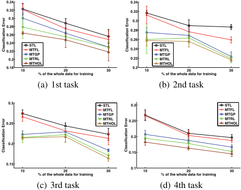
The second one is a multi-domain sentiment classification application 2 . Four binary classification tasks correspond to four domains of products at Amazon.com, which include books, DVDs, electronics and kitchen appliances. For each domain, there are 1000 positive and 1000 negative product reviews corresponding to the two classes of the classification problem. The document representation for each review contains 473856 feature dimensions. Like the above experiments, we use training sets of different sizes for training, corresponding to 10%, 20% and 30% of the data for each task. Classification error is used as the performance measure. For the STL baseline, we use a linear SVM which has been demonstrated to perform well for such text classification applications with high feature dimensionality. For other compared methods, we also use the linear kernel. As above, we perform 10 random data splits and report the mean and standard deviation of the classification error in Figure 1(a) to Figure 1(d). Again, for all settings, MTHOL is either the best or among the best by using paired t-test and ANOVA significance test.
3.3 Examination Score Prediction
This application is a regression problem for predicting the examination scores of the students from 139 secondary schools (http://www.cs.ucl.ac.uk/staff/A.Argyriou/code/). There are
2 http://www.cs.jhu.edu/∼mdredze/datasets/sentiment/
| Method | 1st | 2nd | 3rd | 4th | 5th | 6th | 7th |
|---|---|---|---|---|---|---|---|
| STL | 0.1507 | 0.1920 | 0.1866 | 0.0283 | 0.3563 | 0.6454 | 0.0409 |
| 0.0077 | 0.0087 | 0.0054 | 0.0038 | 0.0246 | 0.0202 | 0.0016 | |
| MTFL | 0.1404 | 0.1953 | 0.1823 | 0.0221 | 0.3294 | 0.6497 | 0.0470 |
| 0.0056 | 0.0079 | 0.0195 | 0.0127 | 0.0139 | 0.0118 | 0.0044 | |
| MTGP | 0.0926 | 0.1471 | 0.1084 | 0.0116 | 0.3465 | 0.6833 | 0.0438 |
| 0.0035 | 0.0076 | 0.0067 | 0.0013 | 0.0070 | 0.0109 | 0.0190 | |
| MTRL | 0.0879 | 0.1358 | 0.1030 | 0.0098 | 0.3248 | 0.6223 | 0.0387 |
| 0.0008 | 0.0038 | 0.0034 | 0.0017 | 0.0054 | 0.0034 | 0.0073 | |
| MTHOL | 0.0782 | 0.1242 | 0.1035 | 0.0082 | 0.3158 | 0.6032 | 0.0372 |
| (t=2) | 0.0019 | 0.0048 | 0.0050 | 0.0015 | 0.0096 | 0.0094 | 0.0042 |
| Method | 1st | 2nd | 3rd | 4th | 5th | 6th | 7th |
| STL | 0.1140 | 0.1714 | 0.1537 | 0.0141 | 0.2805 | 0.5501 | 0.0298 |
| 0.0027 | 0.0032 | 0.0046 | 0.0005 | 0.0062 | 0.0161 | 0.0018 | |
| MTFL | 0.1131 | 0.1800 | 0.1516 | 0.0187 | 0.2832 | 0.5596 | 0.0371 |
| 0.0029 | 0.0050 | 0.0045 | 0.0014 | 0.0081 | 0.0142 | 0.0034 | |
| MTGP | 0.0813 | 0.1208 | 0.0893 | 0.0088 | 0.2982 | 0.5453 | 0.0346 |
| 0.0023 | 0.0058 | 0.0048 | 0.0004 | 0.0093 | 0.0252 | 0.0134 | |
| MTRL | 0.0812 | 0.1122 | 0.0947 | 0.0087 | 0.2712 | 0.5429 | 0.0282 |
| 0.0021 | 0.0032 | 0.0028 | 0.0013 | 0.0031 | 0.0060 | 0.0007 | |
| MTHOL | 0.0706 | 0.0980 | 0.0898 | 0.0078 | 0.1333 | 0.5243 | 0.0200 |
| (t=2) | 0.0029 | 0.0034 | 0.0041 | 0.0016 | 0.0050 | 0.0077 | 0.0027 |
139 learning tasks corresponding to the 139 schools, with a total of 15362 data points. There are 27 input attributes representing information about both the schools and the students. Like the experiment setting on robot inverse dynamics, we use the nMSE as performance measure and kernel ridge regression as the STL baseline. We also use 10% and 20% of the data for training. Table 2 summarizes the results over 10 random data splits. We can see that MTHOL outperforms all other methods.
| Method | 10% | 20% |
|---|---|---|
| STL | 1.0744±0.0235 | 0.9549±0.0116 |
| MTFL | 0.8868±0.0235 | 0.7341±0.0077 |
| MTGP | 0.7267±0.0078 | 0.6282±0.0115 |
| MTRL | 0.7085±0.0160 | 0.5963±0.0194 |
| MTHOL | 0.6889±0.0183 | 0.5717±0.0154 |
3.4 Handwritten Letter Classification
The handwritten letter data set is another classification application (http://multitask.cs.berkeley.edu/). It consists of seven tasks each of which is a binary classification problem for two letters: c/e, g/y, m/n, a/g, a/o, f/t and h/n. The input for each data point consists of 128 features representing the pixel values of the handwritten letter. For each task, there are about 1000 positive and 1000 negative examples. Similar to the multi-domain sentiment classification problem, different settings correspond to 10%, 20% and 30% of the data for training and the performance measure is the classification error. From Table 3, MTHOL again gives very competitive results.
| Method | 10% | 20% | 30% |
|---|---|---|---|
| STL | 0.0949±0.0016 | 0.0794±0.0035 | 0.0765±0.0010 |
| MTFL | 0.0843±0.0073 | 0.0758±0.0045 | 0.0734±0.0024 |
| MTGP | 0.0767±0.0039 | 0.0691±0.0068 | 0.0660±0.0020 |
| MTRL | 0.0733±0.0044 | 0.0615±0.0072 | 0.0601±0.0033 |
| MTHOL | 0.0687±0.0057 | 0.0547±0.0040 | 0.0598±0.0034 |
4 Conclusion
In this paper, we have proposed a novel, nontrivial generalization of an existing multi-task learning method by modeling and learning high-order task relationships.
Although our method can use different values for the degree t, its value has to be set in advance and fixed during model learning. One possible direction to extend the current method is to allow the degree t to be learned from data automatically. To address this issue in our future work, we plan to adopt the full Bayesian approach which may bring about further performance improvement by making model selection via hyperparameter learning as an integral part of model learning.
Acknowledgments
Dit-Yan Yeung has been supported by General Research Fund 621310 from the Research Grants Council of Hong Kong.
@inproceedings{ijcai2013p283,
  title     = {Learning High-Order Task Relationships in Multi-Task Learning},
  author    = {Zhang, Yu and Yeung, Dit-Yan},
  booktitle = {Proceedings of the Twenty-Third International Joint Conference on
               Artificial Intelligence, {IJCAI-13}},
  publisher = {AAAI Press / International Joint Conferences on Artificial Intelligence},
  editor    = {Francesca Rossi},
  pages     = {1917--1922},
  year      = {2013},
  month     = {8},
  url       = {https://ijcai.org/proceedings/2013/283},
}
TY - CPAPER TI - Learning High-Order Task Relationships in Multi-Task Learning AU - Zhang, Yu AU - Yeung, Dit-Yan T2 - Proceedings of the Twenty-Third International Joint Conference on Artificial Intelligence, IJCAI-13 PB - AAAI Press / International Joint Conferences on Artificial Intelligence PY - 2013 SP - 1917 EP - 1922 UR - https://ijcai.org/proceedings/2013/283 ER -Copied
Machine-readable versions of this paper, for tools and AI agents:





