
A Probabilistic Approach to Latent Cluster Analysis
Proceedings of the Twenty-Third International Joint Conference on Artificial Intelligence. Pages 1813-1818.
© 2013 International Joint Conferences on Artificial Intelligence
Abstract
Facing a large number of clustering solutions, cluster ensemble method provides an effective approach to aggregating them into a better one. In this paper, we propose a novel cluster ensemble method from probabilistic perspective. It assumes that each clustering solution is generated from a latent cluster model, under the control of two probabilistic parameters. Thus, the cluster ensemble problem is reformulated into an optimization problem of maximum likelihood. An EM-style algorithm is designed to solve this problem. It can determine the number of clusters automatically. Experimental results have shown that the proposed algorithm outperforms the state-of-the-art methods including EAC-AL, CSPA, HGPA, and MCLA. Furthermore, it has been shown that our algorithm is stable in the predicted numbers of clusters.
- [Azimi and Fern, 2009] Javad Azimi, Xiaoli Z. Fern. Adaptive cluster ensemble selection. In Proceedings of the 21 st International Joint Conference on Artificial Intelligence, pages 993-997, 2009. IJCAI
- [Fern and Brodley, 2003] Xiaoli Z. Fern, and Carla E. Brodley. Random projection for high dimensional data clustering: a cluster ensemble approach. In Proceedings of the 20 th International Conference on Machine Learning, pages 186-193, 2003.
- [Fern and Lin, 2008] Xiaoli Z. Fern, and Wei Lin. Cluster ensemble selection. Statistical Analysis and Data Mining, 1(3): 379-390, 2008
- [Frank and Asuncion, 2010] A. Frank, and A. Asuncion. UCI Machine Learning Repository. Irvine, CA: University of California, School of Information and Computer Science, 2010. [http://archive.ics.uci.edu/ml] Link
- [Fred and Jain, 2005] Ana L.N. Fred, and Anil K. Jain. Combining multiple clusterings using evidence accumulation. IEEE Transactions on Pattern Recognition and Machine Intelligence. 27(6): 835-850, 2005.
- [Jain et al., 1999] Anil K. Jain, M.N. Murty, P.J. Flynn. Data clustering: a review. ACM Computing Surveys, 31(3): 264-323, 1999.
- [Jain, 2010] Anil K. Jain. Data clustering: 50 years beyond K-means. Pattern Recognition Letters, 31(8): 651-666, 2010.
- [MacQueen, 1967] J. MacQueen. Some methods for classifications and analysis of multivariate observations. In Proceedings of the Fifth Berkeley Symposium on Mathematics, Statistics and Probability, University of California Press, pages 281-297, 1967.
- [Manning et al., 2008] Christopher D. Manning, Prabhakar Raghavan, and Hinrich Schutze. Introduction to Information Retrieval, Cambridge UniversityPress, 2008.
- [Minaei-Bidgoli et al., 2004] Behrouz Minaei-Bidgoli, Alexander Topchy, William F. Punch. Ensembles of partitions via data resampling. In Proceedings of International Conference on Information Technology: Coding and Computing (ITCC 2004), pages 188-192, 2004.
- [Strehl and Ghosh, 2002] Alexander Strehl, and Joydeep Ghosh. Cluster ensembles -a knowledge reuse framework for combining multiple partitions. Journal of Machine Learning Research, 3: 583-617, 2002.
- [Vega-Pons and Ruiz-Shulcloper, 2011] Sandro Vega-Pons, and Jose Ruiz-Shulcloper. A survery of clustering ensemble algorithms. International Journal of Pattern Recognition and Artificial Intelligence, 25(3): 337-372, 2011.
References were extracted automatically from the PDF and may contain errors.
Full text extracted automatically from the PDF; figures, tables and equations may differ. The PDF is the version of record.
1 Introduction
The goal of cluster analysis is to discover the underlying structure of a dataset (Jain et al., 1999; Jain, 2010). It normally partitions a set of objects so that the objects within the same group are similar while those from different groups are dissimilar. A large number of clustering algorithms have been proposed, e.g. k-Means, Spectral Clustering, Hierarchical Clustering, Self-Organizing Maps, to name but a few, yet no single one is able to successfully achieve this goal for all datasets. On the same data, different algorithms, or even multiple runs of the same algorithm with different parameters, often lead to clustering solutions that are distinct from each other.
Confronted with a large number of clustering solutions, cluster ensemble or clustering aggregation methods have emerged, which try to combine different clustering solutions into a consensus one, in order to improve the quality of component clustering solutions (Vega-Pons and Ruiz-Shulcloper, 2011). Cluster ensemble methods usually consist of two or three phases: the ensemble generation phase to produce a variety of clustering solutions; then the ensemble selection phase to select a subset of these clustering solutions, which is optional; and finally the consensus phase to induce a unified partition by combining the component ones. In the generation phase, different clustering solutions can be generated by different clustering algorithms, the same algorithm with different parameter settings or initialization, and injection of random disturbance into data set such as data resampling (Minaei-Bidgoli et al., 2004), random projection (Fern and Brodley, 2003), and random feature selection (Strehl and Ghosh, 2002). Following the generation phase, an optional enemble selection phase will select or prune these clustering solutions according to their qualities and diversities (Fern and Lin, 2008; Azimi and Fern, 2009).
In this paper, we focus on the final phase - clustering combination. There are a lot of algorithms for the combination, which can be categorized according to the kind of information exploited. The algorithm proposed here falls into the category making use of the pairwise similarities between objects, which form a co-association matrix in the context of cluster ensembles. Any clustering algorithm can be applied on this new similarity matrix to find a consensus partition. Evidence Accummulation Clustering (Fred and Jain, 2005), or EAC in short, performs a hierarchical clustering of average linkage (AL) or single linkage (SL) on co-associationg matrix, where a maximum lifetime criterion is proposed to determine the number of clusters. Cluster-based Similarity Partitioning (CSPA) algorithm (Strehl and Ghosh, 2002) uses a graph-paritioning algorithm instead, but requires the number of clusters be specified manually. Another algorithm HGPA (Strehl and Ghosh, 2002) can be thought as an approximation to CSPA. Out of this category, MCLA algorithm makes a clustering of clusters based on the similarities between clusters, and then assigns objects to its closest meta-cluster. For a thorough list of related algorithms, please refer to the survey paper by Vega-Pons and Ruiz-Shulcloper (2011).
Although these methods have achieved some success, they are still deficient in several aspects: first, they lack of theoretic underpinning; second, they think that all the clustering solutions be of the same quality, and thus assign the same weight to each clustering solution; last but not the least, most of them (except EAC) require the number of clusters to be specified manually. As to the maximum lifetime criterion adopted by EAC algorithm, it is more or less a rule-of-thumb that is lack of justification. As we shall see in the experiments, the maximum lifetime criterion is unstable in determining the number of clusters.
To tackle these problems, we propose a probabilistic method called LAtent Cluster Analysis, or LACA in short. It assumes that there is a latent cluster model which is unobservable. All the observed Clustering solutions are generated from the latent model under the control of two probabilistic parameters. Our objective is to seek the latent cluster model with the maximum likelihood.
This paper is organized as follows. In Section 2, we introduce the latent cluster model and build its connection with the observed clustering solutions. We devote Section 3 to an EM-style algorithm for inferring the latent cluster model from the observed clustering solutions. In Section 4, we present the experimental results of the proposed method compared with several state-of-the-art cluster ensemble algorithms. Finally, we make the conclusion in Section 5.
2 Latent Cluster Model
Let X = {x1, x2, …, xn} be a set of n objects, where each object xi may be represented as a multidimensional vector, a string, or in any other form. Taking X as input, a clustering algorithm (called clusterer) produces a clustering solution that partitions the n objects into groups. By running clustering algorithms multiple times, we can observe an ensemble of clustering solutions, E = {C 1 , C 2 , …, C |E| }, where each clustering solution C e (1 � e � |E|) partitions the n objects into groups e C e e e c c c | | , , , � .
With respect to a given clustering solution C e , a co-association relationship between two objects xi and xj is defined according to whether they are assigned to the same group:
Two objects xi and xj are said to be co-associated in the clustering solution C e if 1 _ e ij Ο ; otherwise, they are not co-associated.
Given the ensemble of observed clustering solution, what we would like to explore is the latent cluster model. We denote the latent cluster model as / = {Τ1, Τ2, …, Τs}, where Τl (1 η l η s) is a cluster represented as a subset of objects, and s is the real number of clusters. In this paper, we assume that these s latent clusters are non-overlapping, i.e., Τi ⇐ Τj = ⇓ for 1 η i ♦ j η s. Based on the latent cluster model /, we define the co-cluster function for a given pair of objects {xi, xj}:
This latent cluster model serves as the major factor in determining what clustering solutions can be observed, while other factors such as the bias of applied clustering algorithm influences the observed results and leads to some false positives and false negatives.
To build the connection between a clustering solution C e and the latent cluster model /, we introduce two probabilistic parameters:
- ♥ The parameter Ξe to denote the conditional probability that two objects are co-associated in C e given that they are co-cluster in the hidden model /, that is Ξe = Pr( e ij Ο =1|/ij=1); and
- ♥ The parameter re to denote the conditional probability that two objects are co-associated in C e given that they are not co-cluster in the hidden model /, that is re = Pr( e ij Ο =1|/ij=0).
Intuitively, each observed clustering solution provides some evidences about the latent (unobservable) co-cluster relationship between objects. Given a set E of clustering solutions, our objective is to maximize the posterior probability of the latent cluster model /, as follows:
where l(/ | E) = Pr(E | /) is the likelihood function. Assume that these clustering solutions are independent of each other and prior probabilities of all the possible latent cluster models are distributed uniformly, it can be written as the following maximum-likelihood problem:
where l(/ | C e ) = Pr(C e | /) is the likelihood of the latent model / given the observed clustering solution C e (or the probability of observing C e given the latent model /)
The evidence of observing a clustering solution C e can be decomposed into the evidence set of co-association relationships of all object pairs, i.e. whether a pair of objects {xi, xj} are assigned to the same group. Then, we have
Taking logrithm on both sides, we get the log-likelihood:
- � | } | } , {{ | , 1 _ _ / _ / e ij ij j i e and x x n Ο represents the number of object pairs that are co-cluster in the hidden model / and also co-associated in C e ;
- � | } 0 | } , {{ | , 10 _ _ / _ / e ij ij j i e and x x n Ο represents the number of object pairs that are co-cluster in the hidden model, but not co-associated in the observed clustering result C e ;
- � | } 1 0 | } , {{ | , 01 _ _ / _ / e ij ij j i e and x x n Ο represents the number of object pairs that are not co-cluster in the hidden model, but co-associated in the observed clustering result C e ; and
- � | } 0 | } , {{ | , 00 _ _ / _ / e ij ij j i e and x x n Ο represents the number of the object pairs that are not co-cluster in / also not co-associated in the clustering result C e .
By substituting equations (5) or (6) into (4), we can
3 Algorithm Design
Unfortunately, the latent cluster model and the probabilistic parameters of these observed clustering results are all unknown, which make it impossible to seek the solution directly. Here, we proposed an EM-style algorithm to deal with the problem, depicted in Figure 1.
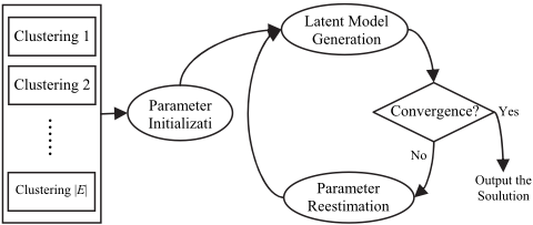
The algorithm consists of four major steps:
- ♥ Step 1 (Parameter Initialization): initialize the probabilistic parameters for each clustering solution;
- ♥ Step 2 (Latent Model Generation): fixing the probabilistic parameters, look for a near-optimal solution (a latent model) to the maximum-likelihood problem with a hill climbing strategy;
- ♥ Step 3 (Parameter Estimation): fixing the latent cluster model, estimate the probabilistic parameters for each clustering solution;
- ♥ Step 4 (Convergence Test): Repeat Step 2 and Step 3 until convergence.
3.1 Parameter Initialization
Given |E| observed clustering solutions C 1 , C 2 , …, C |E| , we use count(xi, xj) to denote the number of clustering solutions where the objects xi and xj are co-associated, and rcount(xi, xj) to denote the number of clustering solutions where xi and xj are not co-associated, that is:
and
It is evident that count(xi, xj) + rcount(xi, xj) = |E| for 1 � i, j η n, i ♦ j.
So far as parameter initialization is concerned, it is taken for granted that different clustering solutions be equally plausible. The higher is the value of count(xi, xj), the more probably the two objects xi and xj are co-clustered. Hence, the two probabilistic parameters for each clustering solution C e is initialized as the following M-estimates:
and
where ESS, standing for "equivalent sample size", is set as 30 by default.
3.2 Latent Model Generation
Once the probabilistic parameters are initialized or re-estimated, the latent cluster model can determined in a hill-climbing manner with respect to value the log likelihood function. Let's start with an empty latent model where each object corresponds to a singleton cluster, and thus any two objects are not co-cluster. Then, we iteratively merge two clusters into a larger one. The selection criterion for merging at each step is described below, step by step.
Let / = {Τ1, Τ2, …, Τt} be the latent cluster model at the current step, and /(uv) be produced by merging Τu and Τv in /. Due to the fact that ) ( , 11 , 11 ) e e n n uv / / 2 = 2 ) ( , 01 , 01 ) ( e e n n uv / / 2 and
Further, it is evident that:
and
Substituting (13) and (14) into (12), we get:
_ / 2 / uv E l E l ) | ( ) | ( ) (
By interchanging the order of summation, it can be derived that:
If we define the affinity score between two objects xi and xj voted by a clustering solution C e as:
we can sum up all the scores voted by C 1 , C 2 , …, C |E| into the corresponding entry M[i, j] of a score matrix M, that is,
Substituting (17) and (18) into (16), we have:
However, using equation (19) directly as the selection criterion may favor merging larger clusters over smaller ones. Thus, we choose to merge two clusters Τs and Τt such that
If we think of the score matrix M as a similarity matrix, the selection criterion is actually the average-linkage (AL). As a result, a hierarchical clustering with average linkage can be applied on the matrix M. What is important is that the elements in the score matrix has clear probabilistic meaning: each element represents actually the log-likelihood ratio of the correponding two objects being co-cluster to being not.
Hidden Model Inference via Hierarchical clustering
By fixing all the parameters Ξe and re (1 η e η |E|), the score matrix M can be constructed according to (17) and (18). The hidden model can be generated by applying the following agglommerative hierarchical clustering on M:
Step 1: We start from the simplest singleton model /0 where each cluster consists of one and only one object.
Step 2: Let t denote the current iteration, and set t = 1.
Step 3: At each iteration t, let / be the cluster model in the previous iteration, i.e., / = /t21. Without loss of generality, we denote /={Τ1, Τ2, …, Τ|/|}. Two clusters Τs and Τt in / are selected according to equation (20).
Step 4: If the average link between Τs and Τt is negative, then terminate the loop and output / as the generated hidden cluster model; otherwise, continue to step 5.
Step 5: The clusters selected at step 3 get merged into a new cluster Τnew = Τs⇒Τt. We update / by removing Τs and Τt, and inserting Τnew. The updated / then serves as the cluster model in the current iteration, that is /t = /.
Step 6: If only two clusters are left, terminate and output /; otherwise, set t = t+1, and go to step 3.
Stopping Criterion: This process is repeated until we can not find a pair of clusters with positive average link (Step 4), or there are only two clusters left (Step 6).
3.3 Parameter Re-estimation
Once a latent cluster model / is generated, it can be used to estimate the probabilistic parameters Ξe and re for each clustering solution C e .
Since the parameter Ξe represents the probability that two objects are co-associated in C e on condition that they are co-cluster in the latent model /, that is, re = Pr(Οe =1|/=1), it can be estimated as:
where the ESS is also set as 30 by default.
Because the parameter re denotes the probability that two objects are co-associated in C e on condition that they are not co-cluster in /, that is re = Pr(Οe =1|/=0), it can be estimated as:
If a clustering solution assigns each object into a distinct group, the corresponding Ξe and re will be both close to 0. On the other extreme, if it assigns all objects into a single group, the corresponding Ξe and re will be both near to 1.
3.4 Convergence Test
Once the probabilistic parameters Ξe and re for each clustering solution C e are re-estimated, we compute the difference between the re-estimated values and the previous ones. If the sum of absolute differences over all clustering solutions is less than a user-specified threshold value, we consider the algorithm as converged and output the latent model.
4 Experiments
We have conducted extensive experiments to compare LACA with several state-of-the-art cluster ensemble methods. Our experiments are designed to demonstrate: 1) LACA is more stable than EAC-AL in determining the number of clusters; 2) LACA outperforms EAC-AL which is also able to determining the number of clusters automatically; 3) A variant verision of LACA, called k-LACA, outperforms CSPA, HGPA and MCLA.
4.1 Experimental Settings
| DataSet | #Object | #Feature | #Class |
|---|---|---|---|
| Iris | 150 | 4 | 3 |
| Glass | 214 | 9 | 6 |
| Ecoli | 336 | 7 | 8 |
| Libras | 360 | 90 | 15 |
| Segmentation | 210 | 19 | 7 |
| Seed | 210 | 7 | 3 |
| Pima | 768 | 8 | 2 |
| Pendigits | 1000 | 16 | 10 |
Data sets. We use eight data sets from the UCI machine learning repository (Frank and Asuncion, 2010) in our experiments. The characteristics of the data sets are summarized in Table 1. Note that, for Pendigits, we randomly select 100 objects from each class.
Cluster Ensemble Generation. We choose to use the K-means algorithm (MacQueen, 1967) as our base clusterer, because of its popularity in many previous cluster ensemble studies. At each run, we generate a cluster ensemble of 200 clustering solutions for a given data set. To be more specific, for a dataset of n objects and m features, each clustering solution is produced as follows:
- ♥ The size s of feature subset is firstly determined by randomly drawing an integer value from the range [minS, maxS], where minS is set to be 3, and maxS is set to be m.
- ♥ A random feature subset FS of size s is generated by drawing s different features from the original m features.
- ♥ An random integer value K is drawn from [minK, maxK], where minK is set to be 2, and maxK is set to be n/15.
- ♥ A clustering solution is obtained by applying K-means algorithm on the dataset, with access to all the objects, but only the s features in FS.
Evaluation Criterion. As all the datasets are labeled, we use the class labels as a surrogate for the true underlying structure of the data. Two commonly used measures, Normalized Mutual Information (NMI) and F-measures, are chosen to evaluate our approach against others.
NMI (Strehl and Ghosh, 2002) treats cluster labels X and class labels Y as random variables and makes a tradeoff between the mutual information and the number of clusters:
where I(⎦) is the mutual information metric and H(⎦) is the entropy metric.
F-measure (Manning et al., 2008) views a clustering solution (on a dataset with n objects) as a series of n(n21)/2 decisions, one for each pair of objects. It makes a compomise between the precision and the recall of these decisions:
4.2 Stability of Predicted Cluster Numbers
To the best of our knowledge, most cluster ensemble methods rely on a user-specified number of clusters. The only exception is the maximum lifetime criterion used in EAC-AL method.
In order to study the stability of our algorithm and EAC-AL in predicted number of clusters, we generate 30 cluster ensembles for each dataset in the way as described in Section 4.1. Our algorithm and EAC-AL are applied on these cluster ensembles to get their predicted cluster numbers. The statistics about these numbers are presented in Table 2. It can be seen from the table that the range [Min, Max] of EAC-AL is much wider than that of LACA on each dataset, suggesting that the cluster numbers predicted by EAC-AL fluctuates a lot for each data set, and especially for Pendigits and Pima. Similar observations can also be made from the standard deviation of cluster numbers on each dataset. We conjecture that this is because life time is not always effective in the prediction of cluster numbers, because the maximum lifetime strategy is more or less a rule of thumb, lack of theoretic justification. As to the average value of the predicted cluster numbers, LACA is larger than EAC-AL on 3 datasets, and smaller on 5, showing inconsistency in some degree.
| Dataset | Method | Min | Max | Average | Std Dev |
|---|---|---|---|---|---|
| Iris | LACA | 3 | 4 | 3.73 | 0.45 |
| EAC-AL | 2 | 4 | 2.73 | 0.98 | |
| Glass | LACA | 5 | 6 | 5.03 | 0.18 |
| EAC-AL | 2 | 6 | 4.40 | 1.65 | |
| Ecoli | LACA | 3 | 5 | 3.73 | 0.83 |
| EAC-AL | 3 | 12 | 4.30 | 2.37 | |
| Libras | LACA | 7 | 9 | 7.70 | 0.70 |
| EAC-AL | 6 | 21 | 11.50 | 5.54 | |
| Segmentation | LACA | 5 | 7 | 5.23 | 0.57 |
| EAC-AL | 2 | 13 | 2.53 | 2.08 | |
| Seed | LACA | 4 | 5 | 4.40 | 0.50 |
| EAC-AL | 2 | 7 | 4.53 | 0.97 | |
| Pima | LACA | 4 | 10 | 8.70 | 1.06 |
| EAC-AL | 4 | 30 | 11.80 | 8.04 | |
| Pendigits | LACA | 10 | 16 | 14.03 | 1.75 |
| EAC-AL | 4 | 48 | 20.53 | 12.27 |
4.3 Comparison with EAC-AL
Table 3 reports the NMI and F-measure values of our algorithm and EAC-AL on the same cluster ensembles. Each value reported here is obtained by averaging across 30 runs. We can see that our algorithm performs better than EAC-AL on 7 out of 8 datasets. The only exception is on the Libras dataset. We conjecture that it is because the average cluster number predicted by EAC-AL is closer to the real number of classes in Libras.
| F-measure | NMI | |||
|---|---|---|---|---|
| Dataset | LACA | EAC-AL | LACA | EAC-AL |
| Iris | 0.8533 | 0.7995 | 0.7535 | 0.7528 |
| Glass | 0.5502 | 0.5395 | 0.3869 | 0.3614 |
| Ecoli | 0.7693 | 0.7545 | 0.6790 | 0.6712 |
| Libras | 0.4267 | 0.4470 | 0.5014 | 0.5333 |
| Segmentation | 0.6091 | 0.4091 | 0.6052 | 0.4617 |
| Seed | 0.8423 | 0.8333 | 0.6680 | 0.6613 |
| Pima | 0.3751 | 0.3597 | 0.0674 | 0.0665 |
| Pendigits | 0.7712 | 0.6809 | 0.7721 | 0.7389 |
4.4 Comparison with CSPA, HGPA and MCLA
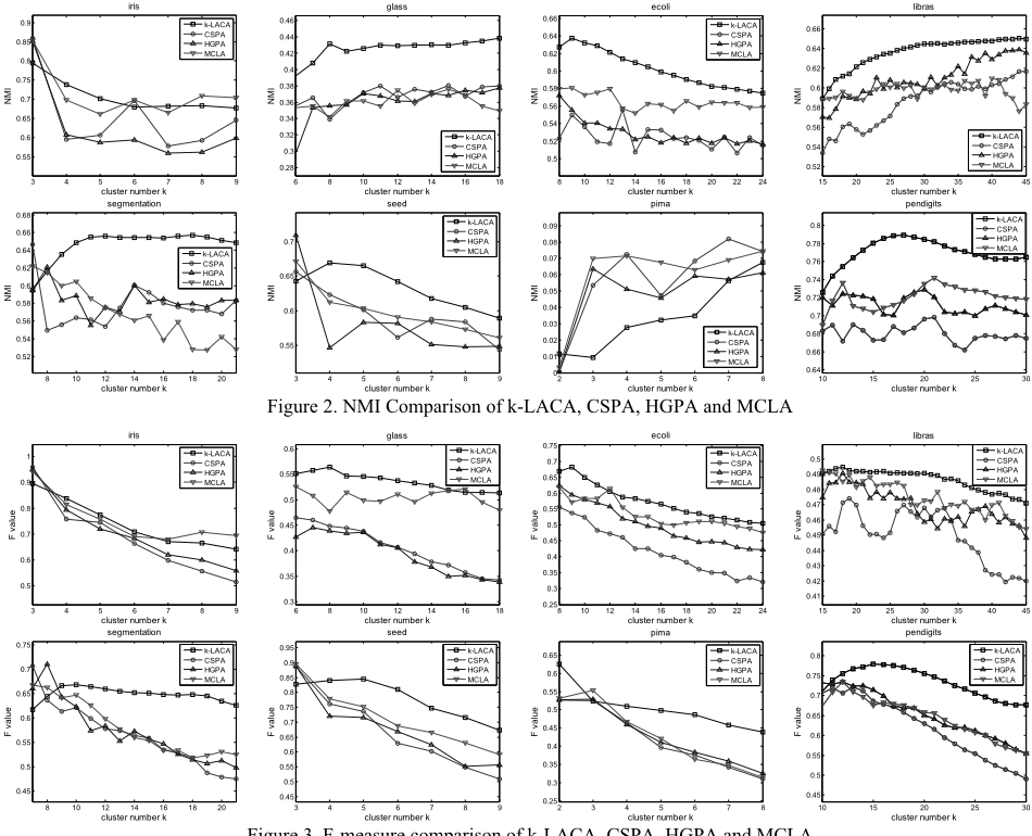
Due to the fact that most existing cluster ensemble methods require a user-specified number of clusters, to make a fair comparison with them, we make a small modification of LACA by accepting a user-specified cluster number k, resulting in a variant version called k-LACA. In k-LACA, when the probabilistic parameters get converged, we force the hierarchical clustering to stop merging only if there are exactly k clusters left, which are then used as the consensus clustering of k-LACA.
On each dataset of l classes, we compare k-LACA with CSPA, HGPA, and MCLA by varying the cluster number k from l to 3×l with step size 1. Figure 2 and Figure 3 depict the NMIs and the F-measures of k-LACA, CSPA, HGPA and MCLA, respectively, which are also avergaed over 30 runs, with different user-specified cluster numbers. It is obvious that the curve of our method is better or at least competitive on almost all the datasets. The only exception is observed on the Pima dataset, where the NMI of our method is lower than the others. Besides, we also find that the curve of our method is more smooth and stable across these different k values. This suggests that our method has achieved high qualities consistently on these levels of hierarchical clustering.
5 Conclusions
In this paper, we proposed a novel cluster ensemble approach by assuming that the observed clustering solutions are generated from a latent cluster model. An EM-style algorithm, called LACA, was designed and implemented to maximize the likelihood function. It has exhibited a satisfactory performance on the experimental datasets, for two reasons: firstly, it can make a stable and reliable prediction of the cluster numbers; secondly, vote of each base clustering solution is weighted which reflects the quality of the base solution.
Acknowledgments
This work is supported by National Airplane Research Program (MJ-Y-2011-39), National Natural Science Fund of China (No. 61170007), Shanghai High-Tech Project (11-43) and Shanghai Leading Academic Discipline Project (No. B114). We are grateful to the anonymous reviewers for their valuable comments.
@inproceedings{ijcai2013p268,
  title     = {A Probabilistic Approach to Latent Cluster Analysis},
  author    = {Xie, Zhipeng and Dong, Rui and Deng, Zhengheng and He, Zhenying and Yang, Weidong},
  booktitle = {Proceedings of the Twenty-Third International Joint Conference on
               Artificial Intelligence, {IJCAI-13}},
  publisher = {AAAI Press / International Joint Conferences on Artificial Intelligence},
  editor    = {Francesca Rossi},
  pages     = {1813--1818},
  year      = {2013},
  month     = {8},
  url       = {https://ijcai.org/proceedings/2013/268},
}
TY - CPAPER TI - A Probabilistic Approach to Latent Cluster Analysis AU - Xie, Zhipeng AU - Dong, Rui AU - Deng, Zhengheng AU - He, Zhenying AU - Yang, Weidong T2 - Proceedings of the Twenty-Third International Joint Conference on Artificial Intelligence, IJCAI-13 PB - AAAI Press / International Joint Conferences on Artificial Intelligence PY - 2013 SP - 1813 EP - 1818 UR - https://ijcai.org/proceedings/2013/268 ER -Copied
Machine-readable versions of this paper, for tools and AI agents:





