Statistical Tests for the Detection of the Arrow of Time in Vector Autoregressive Models

1 Introduction

The detection of causal relations is one of the areas of current interest in the artificial intelligence community [Daniuˇsis et al., 2010][Hoyer et al., 2009][Mooij et al., 2010] [Zhang and Hyv¨arinen, 2009] - [Hoyer et al., 2009][Zhang and Hyv¨arinen, 2009]. Furthermore, the problem of causal discovery has been investigated in other disciplines; namely econometrics, operations research, control theory, and statistics [Granger, 1969][Janzing, 2007]. The reason for the widespread interest in this problem is that unveiling the causal structure of a system allows to determine the mechanisms by which the data are generated. Specifically, causal inference can be used to determine how modifying (not simply measuring) the value of a certain types of variables (the causes) translates into a change in the value for another group of variables (the effects). From a practical viewpoint, understanding cause-effect relations in complex systems allows to perform effective interventions that can be used to modify and control the behavior of the system by manipulating the values of the relevant variables. These effective interventions are useful in different fields of application such as the control of industrial processes, medicine, genetics, epidemiology, economics, social science, meteorology (e.g. the curbing of the trend to global warming), etc. In most cases, causal relations are derived from domain knowledge and incorporated in an ad-hoc manner in the description of the complex system. Another strategy is to discover them by performing interventions in the system. Notwithstanding, interventions are not always possible, they can be expensive or they can be ethically questionable. The question addressed in this investigation is whether causal relations can be automatically induced from unmanipulated empirical data alone. No method of general applicability is available for this purpose. On the contrary, there exist some consistency conditions that need to be fulfilled by the conditional probability distributions of the model variables, which, when used in combination with some reasonable assumptions (e.g. faithfulness), can be used to identify the causal structure of a problem. Conventional methods for causal discovery focus on conditional independences, and since they require observations from at least three variables, they cannot be used for the simple case of a twovariable system in which one is asked to determine whether one of the variables is the cause and the other one the effect.

In this work we analyze the challenging problem of causal discovery in the context of multi-dimensional time-series. As a simplified approach to the general causal inference problem, we consider a specific set up where the variables Xt-1 cause the variables in Xt, in other words, the current value in a multi-variate time series is the effect caused by the preceding values. Specifically, the question analyzed is the following: Given a sample of a stationary multi-variate time series

is this sequence in the correct chronological order or has its time ordering been reversed? For the one-dimensional case it has been shown that under the assumption that the time series is stationary and that it has been generated by an autoregressive model of the form

with non-Gaussian i.i.d noise ϵt, the residuals of a linear model in the backward time direction

are more Gaussian than the corresponding residuals in the forward direction, {ϵt}Tt=1 [Hern´andez-Lobato et al., 2011] .

Under the assumption that the cumulants of the i.i.d noise process exist, the Gaussianization effect associated with the time reversal is translated into a reduction of the magnitude of the cumulants of order higher or equal to 3. Specifically,

where κn(·) denotes the n-th cumulant. For a stationary AR(1) processes with φ ̸= 0 and |φ| < 1 |cn(φ)| < 1 this implies that

Since the cumulants of order higher than two for Gaussian random variables are zero, the cumulants of ˜ ϵt are closer to the cumulants of a Gaussian distribution than the cumulants of ϵt. Therefore, it is possible to say in a precise sense that the distribution of ˜ ϵt is closer to a Gaussian than the distribution of ϵt. In this work we illustrate how the Gaussianization of the residuals of a linear model upon time reversal also occurs for VAR models with non-Gaussian noise. Furthermore, we describe a statistical test based on measures of Gaussianity that can be used to determine the direction of time in time series generated by these models. Our experiments show that the statistical test considered has better predictive performance than previous methods from the literature based on tests of independence [Peters et al., 2009; Gretton et al., 2008].

The organization of the rest of the manuscript is as follows: Section 2 briefly describes vector autoregressive models and gives some evidence supporting the Gaussianization effect associated with the time reversal. Section 3 introduces two statistical tests that can be used to identify the direction of time in a time series generated by a VAR model. These include tests based on independence and tests based on measures of Gaussianity. Section 4 shows the results of several experiments comparing the two methods previously described. Finally, Section 5 gives the conclusions of the paper.

2 Time Reversal in Vector Autoregressive Models

Consider a d-dimensional autoregressive model

where A is a d × d matrix and ϵt is a d-dimensional vector of i.i.d noise. The process is stationary if and only if the eigenvalues of the matrix of autoregressive coefficients, A, are within the unit circle in the complex plane.

If the noise is Gaussian, the time-reversed process is of the form

with ˜ ϵt Gaussian and ˜ ϵt ⊥ Xt+1.

In contrast with the one-dimensional case, the matrix of autoregressive coefficients for the reversed time series, ˜ A, is in general different from the original one, A. Both matrices are related by the similarity transformation

where Σ is the covariance matrix of the time series. Namely,

When the noise is non-Gaussian, it is generally difficult to derive explicit expressions for the time-reversed process, which is non-linear. Nonetheless, one can define the timereversed residuals of a linear fit

It is possible to show that ˜ ϵt is Gaussian and ˜ ϵt ⊥ Xt+1 if and only if ϵt is multi-dimensional Gaussian i.i.d noise. Otherwise, the time-reversed residuals are not Gaussian i.i.d noise. Furthermore, the backward residuals are dependent on the posterior values (in the backward direction of time) of the time series. By analogy to the one-dimensional case [Hern´andez-Lobato et al., 2011], in this work we conjecture that the (multi-dimensional) distribution of backward residuals {˜ ϵt} is more Gaussian than the distribution of forward residuals {ϵt}.

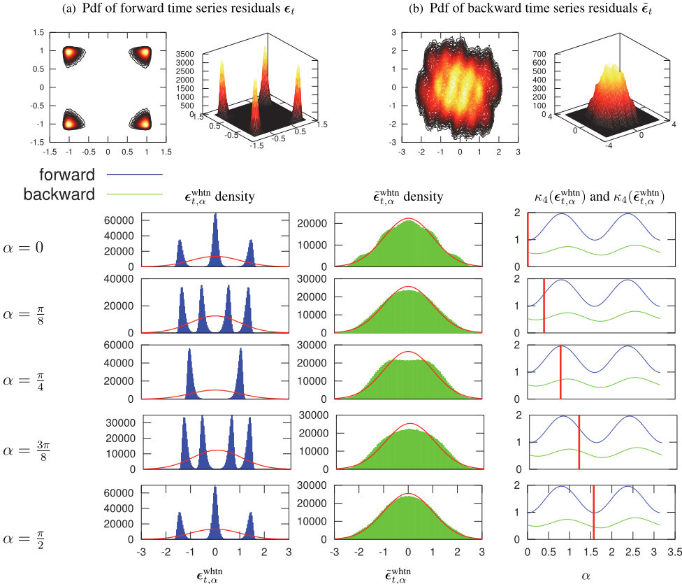
The Gaussianization effect is illustrated for a two dimensional time series in Figure 1. The top-left plot corresponds to the bidimensional pdf of the forward residuals. The top-right plot corresponds to the bidimensional pdf of the backward residuals. The sequence of histograms underneath these plots correspond to one-dimensional marginals of the whitened forward (left) and backward residuals (center) along different projected directions, which are parameterized by an angle α. The plots on the right-most column display the dependence of a measure of deviation from normality (the fourth cumulant) for the one-dimensional marginals as a function of α. On the same column, the vertical red bar shows the value of α used in the projection of the data displayed in left and center columns. These results indicate that similar rules may apply in the multi-variate case to those found for the uni-variate case in [Hern´andez-Lobato et al., 2011]. Namely, the distribution of backward residuals {˜ ϵt} is more Gaussian than the distribution of forward residuals {ϵt}.

3 Statistical Tests for the Detection of the Arrow of Time

Given a time-series generated by a linear VARd(1) process with non-Gaussian i.i.d noise, the observations made so far suggest that two different strategies can be employed to design statistical tests to determine the actual temporal ordering of the series. The first strategy is based on the independence between ϵt and Xt-1, and the dependence between {˜ ϵt} and Xt+1 [Peters et al., 2009]. The second strategy takes advantage of the empirical observation that the residuals of a linear fit in the forward direction are less Gaussian than the residuals in the backward direction.

3.1 Tests Based on Independence

The most direct way to determine the correct chronological ordering of a sequence of values generated by a linear VARd(1) process consists in testing for independence between the residuals of a linear fit and the preceding values both in of the original ordering and in the reversed one. Any measure of independence can be used to implement these types of tests. In this work, we use a test based on embedding of the data in a Hilbert space, the HSIC [Gretton et al., 2008], which has been shown to exhibit excellent performance in simulated and real-world data. Given a sample of N observations of the time series, a N ×N kernel matrix has to be computed. Thus, the cost of this test is quadratic O(N 2 ) in the number of samples. The strategy described will also involve in general two-sample statistical tests.

3.2 Tests Based onMeasures of Gaussianity

The test consists in performing a linear fit for the sequence in the original ordering and in the reversed one. The ordering in which the residuals of the linear fit are less Gaussian is identified as the chronological time ordering. To perform this test one needs a measure of discrepancy with respect to the Gaussian that is applicable to multi-dimensional data and has low computational cost. In particular, consider the twodimensional case. Let ϵ′t = (ϵxt , ϵyt ) be the two components of a bidimensional random vector. The goal is to quantify how different is the distribution of ϵt from a bivariate normal. The following theorem is useful for this purpose:

Theorem 3.1 Let ϵx and ϵy be two random variables. Let Z (α) ≡ ϵx cos α + ϵy sin α. The variable Z (α) is normal ∀α ∈ [0, π] if and only if the joint distribution of ϵx and ϵy is normal.

Therefore, given a one-dimensional measure of the departure of the probability density function f (z) from a Gaussian distribution NG[f (Z )], it is possible to compute a measure of the deviation from the bivariate Gaussian for the distribution of ϵt

In this work we use the absolute value of the fourth cumulant (excess of kurtosis) as the one-dimensional measure of deviation from a Gaussian distribution

The computational cost of this measure is O(N ), i.e., linear in the number of observations.

Note that as opposed to the previous strategy, the strategy described here only involves one-sample statistical tests and is hence expected to perform better in general. Nonetheless, the estimate of the fourth cumulant will deteriorate when the residual distribution is heavy-tailed, as the variance of the estimator will increase significantly. In this situation, more sophisticated measures of non-Gaussianity, such as the maximum mean discrepancy (MMD), can be used at the expense of greater computational complexity (the time complexity of MMD is O(N 2 )) [Gretton et al., 2007].

Equation (11) can be readily extended to more than twodimensions. Unfortunately, the evaluation of the corresponding multi-dimensional integral becomes more expensive. In particular for dimensions larger than three the value of the integral has to be approximated using sampling schemes.

4 Experiments

In this section we carry out experiments with a two-fold purpose. First, to illustrate the statistical properties of the residuals ˜ ϵt that result from fitting a VAR model in the incorrect temporal direction; second, to assess the accuracy of the different statistical tests described in Section 3 to detect the arrow of time of a given sequence of multi-variate ordered values. The experiments involve simulations of two-dimensional V AR2(1) processes

with bidimensional i.i.d. noise ϵ′t = (ϵxt , ϵyt ). The eigenvalues of the matrix of autoregressive coefficients are assumed to be smaller than 1 in absolute value, |λi| < 1, so that the process is stationary. In our experiments different values for λ1 and λ2 within this range are considered. Two different types of additive noise ϵt are also used in the simulations. The first type of noise is of the form

where (Z x t ,Z y t )T ∼ N(0,Σz) for some covariance matrix Σz and rx, ry ∈ (0,∞). In (14), rx and ry determine the level of non-Gaussianity of the marginals, from rx = ry = 1 (fully Gaussian) to rx > 1 and ry > 1 (leptokurtic) or rx < 1 and ry < 1 (platokurtic). Furthermore, Σz allows to introduce dependencies between the two components of ϵt. The second type of noise considered involves normal Gaussian marginals with non-linear dependencies introduced by a Frank copula whose parameter θ determines the level of dependency [Nelsen, 2006]. Namely,

where C (·, ·; θ) denotes a Frank copula with parameter θ and Φ(·) is the cpf of a normal Gaussian distribution. In this case, although the marginals are Gaussian, the joint distribution is non-Gaussian as a consequence of the non-linear dependencies introduced by the copula.

In the experiments described in this section we employ the actual parameters used to generate the data and the actual residuals instead of their corresponding estimates from the observed data. More precisely, in the forward direction we employ as the residual the values of the i.i.d noise ϵt directly. In the reversed time series we compute ˜ ϵt using (10) where ˜A is ˜A = ΣATΣ-1 . Similar results to the ones reported here are obtained when empirical estimates of A and ˜A are used, provided that the samples are large enough so that the estimates of the matrix of autoregressive coefficients are sufficiently accurate.

4.1 Experimental Protocol

The protocol employed in the experiments is very similar to the one used in [Peters et al., 2009; Hern´andez-Lobato et al., 2011]. First, we generate a time series that follows a VARd(p) process. The first τ = 100 log(|λ|)-1 values of the time series are removed in order to ensure that simulated time series is in its stationary regime, where λ is the largest in absolute value among the eigenvalues of the matrix of autoregressive coefficients. Next we compute the empirical residuals for the backward time direction

Then, whitening is applied to residuals. Specifically, given the diagonalization of the covariance matrix of the forward residuals

and the corresponding diagonalization for the backward residuals

the whitened residuals are

where E[ϵwhtn t (ϵwhtn t )′ ] = I and E[˜ ϵwhtn t (˜ ϵwhtn t )′ ] = I. The whitening process guarantees zero mean and a covariance matrix equal to the identity matrix for the distribution of the residuals. Once whitening has been completed, statistical tests are applied to the resulting time series to identify the direction of time, as described in next section.

4.2 No Dependency and Different Levels of non-Gaussianity

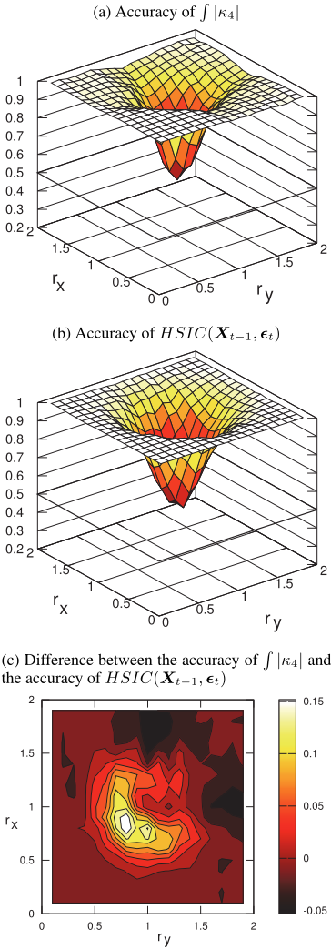
A first experiment compares the performance of the proposed method with the performance of HSIC when ϵt is obtained using (14) and Σz = I. Furthermore, in these experiments we fix λ1 = (√5 - 1)/2 and λ2 = (√5 - 1)/2 which corresponds to the point of maximum discriminative power according to [Hern´andez-Lobato et al., 2011]. P, the matrix that summaries the eigenvectors of A, is set equal to I. Figure 2 shows the accuracy of each method for the detection of the direction of time for different values of rx and ry. As expected, when (rx, ry)T is near (1, 1), the accuracy of the two methods is rather low, although the integral of the fourth cumulant provides better results. By contrast, far from this point, the marginals of the noise become more and more different from a Gaussian and the accuracy of the two methods increases and reaches values near 100%. We also observe that the integral of the fourth cumulant performs worse than the HSIC when one component of ϵt is almost Gaussian and the other is leptokurtic (i.e., rx ≈ 1 and ry ≫ 1 or vice-versa).

4.3 No Dependency and Different Eigenvalues

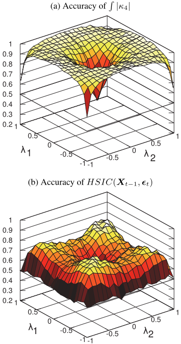
A second experiment investigates the influence of the eigenvalues in the accuracy of each method. For this, the noise of the actual model is generated using (14) with Σz = I and rx = ry = 0.75. The eigenvectors of A are fixed to be P = ( 0 1 -1 0 ). Figure 3 shows the accuracy of each method in this case for the detection of direction of time for different values of λ1 and λ2. We observe that better results are obtained than the ones described in [Hern´andez-Lobato et al., 2011] for a similar one-dimensional experimental setting. This is most likely due to the contribution the two dimensions to the final decision. The figure also shows that the maximum accuracy is achieved for values of λ1 and λ2 near ±(√5 - 1)/2, which is the value of φ that provides the maximum level of Gaussianization in [Hern´andez-Lobato et al., 2011]. In this case, using the integral of the fourth cumulant provides significantly better results than the HSIC for all the values of λ1 and λ2 investigated.

4.4 Non-linear Dependencies but Gaussian Marginals

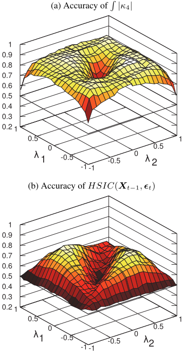
The last experiment considers the influence of the eigenvalues in the accuracy of each method when the noise of the actual model is generated using (15) and θ = 10. That is, the marginals of the noise are Gaussian, but they have nonlinear dependencies introduced by a Frank copula. This case is particularly interesting because the uni-variate techniques described in [Hern´andez-Lobato et al., 2011] will completely fail due to the Gaussianity of the marginals. Specifically, univariate methods cannot determine the direction of time when the marginals of the noise are Gaussian distributed. Figure 4 shows, in this setting, the accuracy of the multi-variate methods described in Section 3. Results are displayed for different values of λ1 and λ2. The figure shows that it is actually possible to detect the direction of time even in the case of having Gaussian marginals as long as the joint distribution of the residuals is non-Gaussian. In this case the integral of the fourth cumulant performs also better than the HSIC.

5 Conclusions and Discussion

We have proposed a statistical test to determine the direction of time of a multi-variate time series generated by a V ARd(1) process based solely on the statistical properties of the data. The test consists in (i) performing a fit to a linear autoregressive model in both the original ordering of the sequence and in the reverse one; (ii) computing the residuals of these linear fits; and (iii) identifying the direction of time as the one in which the residuals are less Gaussian.

A measure of discrepancy between the distribution of the residuals of the time series from a multi-variate Gaussian distribution has been defined. This measure is computed using several projections of the data and an average of the deviation of the projected data from a one-dimensional Gaussian distribution. The efficiency of the test proposed has been evaluated in several experiments involving bidimensional VARd(1) processes (d = 2), with different types of non-Gaussian noise and different values of {λi}di=1 , i.e., the eigenvalues of the matrix of autoregressive coefficients. The test is very efficient when the distribution of the noise is highly non-Gaussian. The strongest Gaussianization effect occurs for values of |λ| close to √5-1 2 , the golden ratio conjugate [Hern´andez-Lobato et al., 2011].

In our experiments the methods based on tests for Gaussianity show better performance than tests based on independence. Furthermore, they are more computationally efficient. In particular, the tests for Gaussianity scale linearly with the number of samples while the tests based on independence scale quadratically. The better performance of tests based on measures of Gaussianity is likely due to the fact that these tests are one-sample tests while independence tests are two-sample tests. Specifically, tests for Gaussianity calculate a distance between the residuals in each direction, i.e., {ϵt} and {˜ ϵt}, and the Gaussian distribution. On the contrary, independence tests compute independence measures between Xt-1 and ϵt, and then between Xt+1 and ˜ ϵt. Thus, in general they are expected to be more sensitive to fluctuations in the data.

Finally, we note that the goal in causal discovery is to determine whether variable X causes variable Y or vice-versa. A particular case of this problem is precisely determining the direction of time. If X and Y are identically distributed random variables and the relation between them is linear, the analysis carried out in this work for time series is also valid for determining whether X causes Y . Thus, we expect that the method described in this paper can also be applied to more general problems of causal discovery.

Acknowledgment

Daniel Hern´andez-Lobato and Alberto Su´arez acknowledge support from the Spanish MCyT (Project TIN2010-21575-C02-02).