
Thinking of Images as What They Are: Compound Matrix Regression for Image Classification
Proceedings of the Twenty-Third International Joint Conference on Artificial Intelligence. Pages 1530-1535.
© 2013 International Joint Conferences on Artificial Intelligence
Abstract
In this paper, we propose a new classification framework for image matrices. The approach is realized by learning two groups of classification vectors for each dimension of the image matrices. One novelty is that we utilize compound regression models in the learning process, which endows the algorithm increased degree of freedom. On top of that, we extend the two-dimensional classification method to a semi-supervised classifier which leverages both labeled and unlabeled data. A fast iterative solution is then proposed to solve the objective function. The proposed method is evaluated by several different applications. The experimental results show that our method outperforms several classification approaches. In addition, we observe that our method attains respectable classification performance even when only few labeled training samples are provided. This advantage is especially desirable for real-world problems since precisely annotated images are scarce.
- [Belkin et al., 2006] Mikhail Belkin, Partha Niyogi, and Vi- kas Sindhwani. Manifold regularization: A geometric framework for learning from labeled and unlabeled ex- amples. Journal of Machine Learning Research, 12:2399- 2434, 2006.
- [Cai et al., 2007] Deng Cai, Xiaofei He, and Jiawei Han. Semi-supervised discriminant analysis. In ICCV, pages 1- 7, 2007.
- [Cao et al., 2013] Xiaochun Cao, XingxingWei, Yahong Han, Yi Yang, and Dongdai Lin. Robust tensor cluster- ing with non-greedy maximization. In IJCAI, 2013. IJCAI
- [Cohen et al., 2004] Ira Cohen, Fabio Gagliardi Cozman, Nicu Sebe, Marcelo Cesar Cirelo, and Thomas S. Huang. Semisupervised learning of classifiers: The- ory, algorithms, and their application to human-computer interaction. IEEE Trans. Pattern Anal. Mach. Intell., 26(12):1553-1567, 2004.
- [Fergus et al., 2010] Robert Fergus, Hector Bernal, Yair Weiss, and Antonio Torralba. Semantic label sharing for learning with many categories. In ECCV (1), pages 762- 775, 2010.
- [Fukunaga, 1990] Keinosuke Fukunaga. Introduction to stat- istical pattern recognition (2nd ed.). Academic Press Pro- fessional, San Diego, USA, 1990.
- [Gourier et al., 2004] Nicolas Gourier, Daniela Hall, and James L. Crowley. Estimating face orientation from ro- bust detection of salient facial features. In ICPR, Inter- national Workshop on Visual Observation of Deictic Ges- tures, 2004.
- [He et al., 2005] Xiaofei He, Deng Cai, and Partha Niyogi. Tensor subspace analysis. In NIPS, 2005.
- [Hou et al., 2013] Chenping Hou, Feiping Nie, Dongyun Yi, and Yi Wu. Efficient image classification via multiple rank regression. IEEE Transactions on Image Processing, 22(1):340-352, 2013.
- [Jolliffe, 2002] Ian T. Jolliffe. Principal Component Analysis (2nd ed.). Springer-Verlag, New York, USA, 2002.
- [Kong et al., 2005] Hui Kong, Lei Wang, Eam Khwang Teoh, Jian-Gang Wang, and Ronda Venkateswarlu. A framework of 2D Fisher discriminant analysis: Applic- ation to face recognition with small number of training samples. In CVPR (2), pages 1083-1088, 2005.
- [Liu et al., 2013] Xiao Liu, Mingli Song, Dacheng Tao, Luming Zhang, Jiajun Bu, and Chun Chen. Semi- supervised node splitting for random forest construction. In CVPR, 2013.
- [Ma et al., 2011] Zhigang Ma, Yi Yang, Feiping Nie, Jasper R. R. Uijlings, and Nicu Sebe. Exploiting the entire fea- ture space with sparsity for automatic image annotation. In ACM Multimedia, pages 283-292, 2011.
- [Nene et al., 1996] Sameer A. Nene, Shree K. Nayar, and Hiroshi Murase. Columbia object image library (coil-20). In Technical Report CUCS-005-96, Columbia University, 1996.
- [Pirsiavash et al., 2009] Hamed Pirsiavash, Deva Ramanan, and Charless Fowlkes. Bilinear classifiers for visual re- cognition. In NIPS, pages 1482-1490, 2009.
- [Saberian et al., 2011] Mohammad J. Saberian, Hamed Masnadi-Shirazi, and Nuno Vasconcelos. Taylorboost: First and second-order boosting algorithms with explicit margin control. In CVPR, pages 2929-2934, 2011.
- [Sharma et al., 2010] Avinash Sharma, Etienne von Lavante, and Radu Horaud. Learning shape segmentation us- ing constrained spectral clustering and probabilistic label transfer. In ECCV (5), pages 743-756, 2010.
- [Vasilescu and Terzopoulos, 2003] M. Alex O. Vasilescu and Demetri Terzopoulos. Multilinear subspace analysis of im- age ensembles. In CVPR (2), pages 93-99, 2003.
- [Wang and Ahuja, 2005] Hongcheng Wang and Narendra Ahuja. Rank-r approximation of tensors: Using image- as-matrix representation. In CVPR (2), pages 346-353, 2005.
- [Xu et al., 2005] Dong Xu, Shuicheng Yan, Lei Zhang, HongJiang Zhang, Zhengkai Liu, and Heung-Yeung Shum. Concurrent subspaces analysis. In CVPR (2), pages 203-208, 2005.
- [Yang et al., 2004] Jian Yang, David Zhang, Alejandro F. Frangi, and Jing-Yu Yang. Two-dimensional PCA: A new approach to appearance-based face representation and recognition. IEEE Trans. Pattern Anal. Mach. Intell., 26(1):131-137, 2004.
- [Yang et al., 2012] Yi Yang, Feiping Nie, Dong Xu, Jiebo Luo, Yueting Zhuang, and Yunhe Pan. A multimedia re- trieval framework based on semi-supervised ranking and relevance feedback. IEEE Trans. Pattern Anal. Mach. In- tell., 34(4):723-742, 2012.
- [Yang et al., 2013] Yi Yang, Jiangkuan Song, Zi Huang, Zhigang Ma, Nicu Sebe, and Alexander G. Hauptmann. Multi-feature fusion via hierarchical regression for mul- timedia analysis. IEEE Transactions on Multimedia, 15(3):572-581, 2013.
- [Ye et al., 2004] Jieping Ye, Ravi Janardan, and Qi Li. Two- dimensional linear discriminant analysis. In NIPS, 2004.
- [Yin et al., 2006] Lijun Yin, Xiaozhou Wei, Yi Sun, Jun Wang, and Matthew J. Rosato. A 3D facial expression database for facial behavior research. In FG, pages 211- 216, 2006.
- [Zhang et al., 2011] Lei Zhang, Meng Yang, and Xiangchu Feng. Sparse representation or collaborative representa- tion: Which helps face recognition? In ICCV, pages 471- 478, 2011.
- [Zhu et al., 2003] Xiaojin Zhu, Zoubin Ghahramani, and John D. Lafferty. Semi-supervised learning using gaussian fields and harmonic functions. In ICML, pages 912-919, 2003.
- [Zhu, 2007] Xiaojin Zhu. Semi-supervised learning literat- ure survey. In Technical Report 1530, University of Wis- consin, Madison, 2007.
References were extracted automatically from the PDF and may contain errors.
Full text extracted automatically from the PDF; figures, tables and equations may differ. The PDF is the version of record.
1 Introduction
Several works have indicated that matrix form may be a more natural representation of an image to reflect its 2D structure [Ye et al., 2004][Yang et al., 2004][Kong et al., 2005][Pirsiavash et al., 2009][Cao et al., 2013]. Typical examples include objects, faces and handwritten digits. However, most existing classification algorithms require that an image be represented by a vector, which is normally obtained by concatenating each row (or column) of an image matrix.
The vectorization of an image has some drawbacks. First, the spatial correlation of the image is broken. Second, it causes the dimensionality increase in multiplication effect, and thus heavily increased computational complexity. The curse of dimensionality additionally causes the over-fitting problem if we use a small number of examples to train the classifiers.
Aiming to preserve the correlation within the image matrix while reducing the computation complexity, researchers have proposed two-dimensional based analyzing methods for images that are better represented as matrices [Ye et al., 2004][Yang et al., 2004][Kong et al., 2005]. A well known
Feiping Nie
University of Texas at Arlington, USA feipingnie@gmail.com Nicu Sebe University of Trento Italy sebe@disi.unitn.it
approach within this paradigm is the two-dimensional subspace learning based classification. This approach is normally achieved by a two-step process. First, it eliminates noise and redundancy from the original data by projecting the data into a lower dimensional subspace. Then it applies classifiers on the low dimensional data for classification. A merit is that both computational efficiency and classification accuracy can be obtained. Classical works include the two-dimensional LDA [Ye et al., 2004] extended from Linear Discriminant Analysis (LDA) [Fukunaga, 1990], twodimensional PCA [Yang et al., 2004] extended from Principle Component Analysis (PCA) [Jolliffe, 2002], etc.
Besides these two-dimensional methods, researchers have also developed tensor subspace analysis algorithms [Vasilescu and Terzopoulos, 2003][Wang and Ahuja, 2005][He et al., 2005][Xu et al., 2005] which can handle even more dimensions. These methods can be readily employed for image matrices by setting the tensor order to two. Typical tensor based subspace learning methods include Tensor LGE [He et al., 2005], Tensor LPP [He et al., 2005] and so on.
The aforementioned methods are able to preserve the spatial correlation of an image and to avoid the curse of dimensionality. Nonetheless, for classification they require a nonconvenient two-step process, i.e., subspace learning followed by different classifiers. Although the first step processes image matrices directly, the classifying step still requires the data to be vectorized. Besides, the separation of subspace learning and classification does not guarantee the classifiers benefit the most from the learned subspace. Recently, Pirsiavas et al. [Pirsiavash et al., 2009] have proposed a bilinearSVM classifier which is able to classify image matrices in an integrated framework and Hou et al. have proposed a regression model for matrix data classification in [Hou et al., 2013]. These approaches are encouraging, however, they need many labeled training data but labeled data are expensive to acquire. The over-fitting problem is likely to occur when the number of training data remains small. It would be more appealing if a classifier classifies image matrices with good performance by using only limited labeled training samples. This is precisely what we want to do in this paper.
Previous work has shown that if properly designed, semisupervised learning [Zhu, 2007] is able to attain improved performance for many applications by using a small amount of labeled training data [Cohen et al., 2004][Liu et al., 2013][Yang et al., 2013][Ma et al., 2011]. A popular approach to realize semi-supervised learning is by building the graph Laplacian. For instance, Yang et al. have proposed a semi-supervised ranking scheme by learning a robust Laplacian matrix through Local Regression and Global Alignment [Yang et al., 2012]. Cai et al. have proposed a semi-supervised dimensionality reduction algorithm called Semi-supervised Discriminant Analysis (SDA) in [Cai et al., 2007]. In [Fergus et al., 2010], Fergus et al. have integrated graph Laplacian into a semi-supervised semantic label sharing method for learning with many categories. Sharma et al. [Sharma et al., 2010] present a new constrained spectral clustering method that builds upon graph Laplacian embedding to propagate pairwise constraints and to cluster the data for shape segmentation.
Inspired by the progress of two-dimensional analysis and semi-supervised learning, we propose a new classification scheme for image matrices. The proposed method leverages two groups of classification vectors with compound regression models, and the graph Laplacian based semi-supervised learning jointly for classification. Semi-supervised learning enables our method to leverage both labeled and unlabeled data. The proposed method thereby overcomes the deficiency of [Pirsiavash et al., 2009].
Another novelty of our method is that it exploits compound regression models. This is different from traditional single regression model as several regression models are integrated. In this way, these regression models work collaboratively for the learning process, which provides us with a larger space to find the optimal solution. In other words, the degree of freedom is increased. The classification performance can be enhanced subsequently.
We name the new method Semi-supervised Twodimensional Classification (SSTC). The main contributions of our work are summarized as:
- SSTC can conduct classification directly using the data in matrix form. The image 2D structure is intact in our framework so that the spacial correlation is preserved. Additionally, the efficiency is guaranteed by avoiding the generation of high-dimensional vectors and the flexibility is increased by using compound regression models.
- Our method is implemented in the semi-supervised scenario, which utilizes both labeled and unlabeled data for classification. It is cost-saving and at the same time is able to prevent over-fitting few labeled training data.
- The experiments on different applications show that our method yields good results even when few labeled samples are available. This attribute is attractive for realworld applications since labeled training data are difficult to obtain.
2 Classifying Image Matrices
In this section, we present the formulation of our Semisupervised Two-dimensional Classification (SSTC) framework followed by a detailed solution for solving the objective function.
2.1 Learning Two Groups of Classification Vectors
Classification aims to learn a predictor f that for an input datum x predicts an output y. For traditional classification algorithms, x is a vector representation of an image. f is decided by minimizing the following regularized empirical error based on a set of training data {xi, yi}ni=1 where yi indicates the label of xi:
loss(·) is a loss function and Ω(f) is the regularization function on f with µ as its parameter.
Among others, ridge regression has shown to be effective for classifying vector data. Denoting X = [x1, x2, · · · , xn] ∈ Rd×n as the training set, the objective function of traditional ridge regression is then defined as
where wj |cj=1 ∈ Rd×1 are used to classify each datum xi into c different classes.
Different from traditional way which copes with vector data, we propose to classify image matrices directly. To begin with, we denote X = [X1,X2, · · · ,Xn] ∈ Rp×q×n as the training set where Xi ∈ Rp×q (1 ≤ i ≤ n) is the i-th datum and n is the total number of the training data. Let Y = [y1, y2, ..., yn] ∈ {0, 1}c×n be the labels. yr i denote the r-th datum of yi and yr i = 1 if Xi is in the r-th class, while yr i = 0 otherwise.
Eq. (2) indicates that the training process for wj|cj=1 is actually c separate procedures. In this sense, we consider classifying Xi|ni=1 to each class separately. Inspired by [Hou et al., 2013], for the r-th class we use two groups of classification vectors uj|mj=1 ∈ Rp×1 and vj|mj=1 ∈ Rq×1 and rewrite Eq. (2) as:
m(m > 1) indicates that we have m compound regression models. Compared with single regression model, i.e., m = 1, using compound regression models provides us with larger space to search for the solution.
To step further, we extend Eq. (3) to a semi-supervised scenario using the graph Laplacian. We first define an affinity matrix A whose element Aij reflects the similarity between Xi and Xj as
The graph Laplacian is then constructed through L = D -G where L is the graph Laplacian matrix and D is a diagonal matrix with Dii = ∑nj=1 Aij .
Suppose l data are labeled in the training set, i.e., ∀i > l, yi|ni=l+1 = 0c×1 . For semi-supervised learning, l is usually much smaller than n. To avoid being heavily dependent on the few labels provided with the labeled training data, we bring in a predicted label vector f r = [f r 1 , . . . , f rn ] ∈ R1×n for all the training data where f r i is the predicted label value of Xi ∈ X. f r should be consistent with the known labels of the training data and be smooth on the graph Laplacian so it can be optimized through the following objective function [Zhu et al., 2003][Zhu, 2007]:
where Tr (·) denotes the trace operator; S is a selection matrix whose diagonal element Sii = ∞ if Xi is labeled and Sii = 1 otherwise; yr = [yr 1 , ..., yr l , 0, ..., 0] ∈ R1×n is the ground truth labels of the training data.
By incorporating Eq. (4) into Eq. (3), we propose our objective function for the r-th class as:
2.2 Optimization
We propose an iterative approach to solve the objective problem of Eq. (5).
we have:min
where Tr (·) denotes the trace operator and Gv = (λBBT + µDv)-1 . Setting the derivative of Eq. (8) w.r.t. u to 0, we have
Algorithm 1: Optimizing the classification vectors uj|mj=1 and vj|mj=1 .
Data: Training data X ∈ Rp×q×n
Training data labels Y ∈ Rc×n
Parameters λ and µ.
Result: Converged uj|mj=1 and vj|mj=1 for c classes. begin
Compute the graph Laplacian matrix L ∈ Rn×n Compute the decision matrix S ∈ Rn×n
Setting the derivative of Eq. (10) w.r.t. f r to 0, we obtain:
where In denotes an n × n identity matrix and Ev = (L + S-λ2BT GvB+λIn)-1 . Substituting Eq. (9) with Eq. (11), we have:
u = λGvBEvS(yr )T
which can be easily converted to uj|mj=1 .
(12)
⎡⎣ uT1 u1Iq ... uTmumIq ⎤⎦ where Iq ∈ Rq×q is an identity matrix. Then Eq. (5) becomes:
Setting the derivative of Eq. (13) w.r.t. v to 0, it becomes
where Gu = (λCCT + µDu)-1 . By substituting v into Eq. (13) and setting its derivative w.r.t. f r to 0, we get:
where Eu = (L + S - λ2C T GuC + λIn)-1 . Consequently, we obtain
and then vj|mj=1 .
The optimization of uj|mj=1 , vj|mj=1 and f r is iterated until convergence. The detailed iteration process is given in Algorithm 1.
Once the u and v for each class are obtained, we can easily get the two groups of classification vectors uj|mj=1 and vj |mj=1 . Then we propose Algorithm 2 to predict the labels of the testing data.
Algorithm 2: The classification process.
Data: Testing data Xte ∈ Rp×q×nte
Classification vectors uj|mj=1 and vj|mj=1 for c
classes
Result: Predicted labels Y pre of the testing data.
begin
By the following theorem, we can verify that the proposed iterative approach in Algorithm 1 converges and the global solutions of uj|mj=1 and vj|mj=1 are obtained.
Theorem 1 The objective function value shown in (5) monotonically decreases in each iteration until convergence using the iterative approach in Algorithm 1.
To prove Theorem 1, we first give the following lemma:
Lemma 1 By fixing vj|mj=1 , we obtain the global solutions for uj|mj=1 and f r . In the same manner, by fixing uj|mj=1 , we obtain the global solutions for vj|mj=1 and f r .
Proof. By fixing vj|mj=1 , the objective function in Eq. (5) is converted to the problem in Eq. (8). It can be seen that Eq. (8) is a convex optimization problem w.r.t. uj|mj=1 and f r . Therefore, we can obtain the global solutions for uj|mj=1 and f r by setting the derivative of Eq. (8) w.r.t. them to zero respectively. Based on the similar theory, we also prove that by fixing uj|mj=1 , we obtain the global solutions for vj|mj=1 and f r □.
Next, we prove Theorem 1 as follows:
Proof.Suppose after the t-th iteration, we obtain utj ∣∣mj=1 , vt j ∣∣mj=1 and f r t . In the next iteration, we fix vj|mj=1 as vt j ∣∣mj=1 and solve for ut+1 j ∣∣mj=1 and f r t+1 . According to Lemma 1, we obtain:
Similarly, when we fix uj|mj=1 as utj ∣∣mj=1 the following inequality holds:
By integrating Eq. (17) and Eq. (18), we have:
Eq. (19) demonstrates that the objective function value decreases after each iteration. Thus, we have proved Theorem 1 □.
3 Experiments
In this section, we apply SSTC to facial expression recognition, face recognition, head pose estimation, object recognition and handwritten digit recognition. We compare SSTC to 7 algorithms which are 2DLDA [Ye et al., 2004], Tensor LPP (T-LPP) [He et al., 2005], BilinearSVM [Pirsiavash et al., 2009], TaylorBoost [Saberian et al., 2011], CRC-RLS [Zhang et al., 2011], Semi-supervised Discriminant Analysis (SDA) [Cai et al., 2007] and Manifold Regularization (MR) [Belkin et al., 2006]. The performance is evaluated by accuracy.
The settings of the experiments are as follows: 1) The grey pixel values of the images are used as features. SSTC, 2DLDA, T-LPP and BilinearSVM deal with image matrices while other methods use vectors. 2) Some parameters need to be set. One of them is the parameter k that specifies the k nearest neighbors used to compute the graph Laplacian matrix L. We fix it at 10 empirically. The number of regression models m is fixed at 3 empirically for all the experiments. The regularization parameters, denoted as λ and µ in Eq. (5), are tuned from {10-4 , 10-2 , ..., 102 , 104}. We similarly tune all the regularization parameters for other methods (if any). The best results from the optimal parameters are reported for all the methods. 3) Each dataset is randomly split into two subsets, one as the training set whereas the other as the testing set. 10% training data are labeled. The split is conducted 5 times independently and we report the average results.
3.1 Datasets
We first introduce the datasets used in our experiments.
Facial Expression Recognition: The BU-FE (Binghamton University Facial Expression) database [Yin et al., 2006] is used. It consists of 2500 images of seven facial expressions. The images were cropped to 32 × 32. We randomly select 1000 images as the training data and the remaining images as the testing data.
Face Recognition: The UMIST face database 1 is used. The database consists of 575 face images from 20 different subjects. Each image was resized to 28×23. We randomly select 400 images as the training set and the remaining images as the testing set.
Head Pose Estimation: We use the Pointing'04 database [Gourier et al., 2004]. It comprises 2790 images from 15 different people. Each image was resized to 40 × 30. Every head pose is determined by both pan and tilt angles. For pan, the angle varies between -90 and +90 degrees with a step of 15 degrees, resulting in 13 poses. Whereas for tilt, the angle varies as -90, -60, -30, -15, 0, +15, +30, +60, +90 degrees to generate 9 poses. We evaluate the performance on both pan and tilt estimation. For both experiments, 1000 images are randomly chosen as the training data and the rest are the testing data.
Object Recognition: We use the Coil20 dataset [Nene et al., 1996]. Coil20 includes 1440 grey scale images with 20 different objects. The images were resized to 32 × 32. We use 500 images as the training data and the rest as the testing data.
Handwritten Digit Recognition: We use the USPS database to evaluate the performance on handwritten digit recognition. The database contains 9298 gray-scale handwritten digit images. The images were resized to 16 × 16. 1000 images are randomly selected as the training set and the remaining images are the testing data.
1 http://images.ee.umist.ac.uk/danny/database.html
3.2 Experimental Results
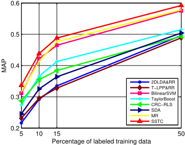
The performance comparison of different algorithms are presented in Table 1. It can be seen that our method SSTC is consistently the best algorithm for different applications. We also conduct an experiment to study the performance variance w.r.t. 5%, 10%, 15% and 50% labeled training data taking facial expression recognition as an example. The result is displayed in Figure 1.
From the experimental results, we observe that 1) SSTC is consistently the best classification algorithm. 2) As the number of labeled training data increases, the performance of all methods is improved. 3) SSTC, BilinearSVM and MR gain the top performance for all settings, which indicates that preserving image 2D structure and semi-supervised learning both contribute to the performance. 4) When 50% training data are labeled, the advantage of SSTC and MR over other supervised algorithms (except BilinearSVM) decreases noticeably. MR is worse than BilinearSVM. The phenomenon demonstrates that supervised algorithms are preferable when we have a large amount of labeled training data. 5) When less than 50% training data are labeled, SSTC and MR generally have more advantage over other supervised algorithms (except BilinearSVM). SSTC is visibly better than Bilinear SVM when 5% training data are labeled and MR is competitive with BilinearSVM. It indicates that through proper design, semi-supervised approaches do benefit much from the usage of unlabeled data.
3.3 Compound RegressionModels vs Single Regression Model
Our algorithm uses compound regression models for classification. In the previous experiments, the number of regression models m was fixed at 3. To show its advantage over single regression model, we reduce m to 1 in this experiment.
Table 2 shows the classification results by using compound regression models (m = 3) and using single regression model (m = 1). We can see that using compound regression models results noticeable performance gain (from 5.4% to 17.6%
| Dataset | 2DLDA | T-LPP | BilinearSVM | TaylorBoost | CRC-RLS | SDA | MR | SSTC |
|---|---|---|---|---|---|---|---|---|
| BU-FE | 29.2% | 29.5% | 41.2% | 36.6% | 36.4% | 32.5% | 41.4% | 43.5% |
| UMIST | 59.8% | 66.3% | 61.7% | 54.3% | 59.2% | 64.6% | 65.6% | 68.1% |
| Pointing'04 | 31.4%(Pan) 10.7%(Tilt) | 33.3%(Pan) 12.1%(Tilt) | 30.6%(Pan) 15.7%(Tilt) | 34.8%(Pan) 15.8%(Tilt) | 32.1%(Pan) 16.6%(Tilt) | 31.1%(Pan) 15.7%(Tilt) | 35.3%(Pan) 16.9%(Tilt) | 36.0%(Pan) 17.4%(Tilt) |
| Coil20 | 59.1% | 70.8% | 71.7% | 66.0% | 72.1% | 75.0% | 74.8% | 76.8% |
| USPS | 73.0% | 71.8% | 78.3% | 78.9% | 75.7% | 76.6% | 78.3% | 81.8% |
| BU-FE | UMIST | Pointing'04 | Coil20 | USPS | |
|---|---|---|---|---|---|
| Single | 40.6% | 64.6% | 33.4%(Pan) 14.8%(Tilt) | 70.2% | 75.7% |
| Compound | 43.5% | 68.1% | 36.0%(Pan) 17.4%(Tilt) | 76.8% | 81.8% |
| Relative Improvement | 7.1% | 5.4% | 7.8%(Pan) 17.6%(Tilt) | 9.4% | 8.1% |
on different datasets). This validates that using compound regression model is advantageous as we have larger space to search for the optimal solution. Therefore, the performance can be improved.
3.4 Parameter Sensitivity &Convergence
In this part, we study the performance variance w.r.t. the regularization parameters λ and µ. Then an experiment on convergence is presented.
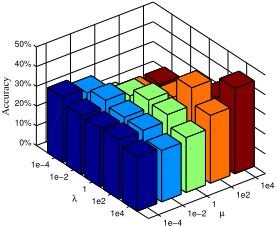
We use the BU-FE dataset for the experiments. Figure 2 shows the parameter sensitivity and we learn that better results are normally obtained when λ and µ are comparable. Figure 3 shows how fast Algorithm 1 converges for one class on this dataset by fixing the parameters at the optimal values when the best classification result is obtained. We observe that for the specified setting Algorithm 1 converges with 4 iterations, which is very fast.
4 Conclusion
Representing images with matrices is better in preserving the spatial correlation and avoiding the curse of dimensionality. We have proposed a method to classify image matrices, which is realized by learning two groups of classification vectors for each dimension of the images. Our method is a Iteration Number semi-supervised algorithm which uses both labeled and unlabeled data. An efficient iterative algorithm has also been proposed to solve our objective function. Our method processes the image matrices directly to capture the spatial correlation and achieves good results when using few labeled training samples, which is cost-saving. The major novelty of our method is that it uses compound regression models. By using compound regression models, we have a larger space to search for the optimal solution, resulting in improved performance. Experiments on different applications were further conducted to evaluate the efficacy of our method. The results are encouraging and have demonstrated that our method is especially competitive when only few labeled training data are available.
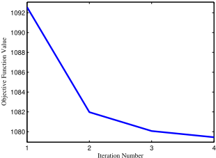
Figure 3: Convergence.
Acknowledgments
This paper was partially supported by the National Program on Key Basic Research Project of China (973 Program) under grant 2010CB327903.
@inproceedings{ijcai2013p228,
  title     = {Thinking of Images as What They Are: Compound Matrix Regression for Image Classification},
  author    = {Ma, Zhigang and Yang, Yi and Nie, Feiping and Sebe, Nicu},
  booktitle = {Proceedings of the Twenty-Third International Joint Conference on
               Artificial Intelligence, {IJCAI-13}},
  publisher = {AAAI Press / International Joint Conferences on Artificial Intelligence},
  editor    = {Francesca Rossi},
  pages     = {1530--1535},
  year      = {2013},
  month     = {8},
  url       = {https://ijcai.org/proceedings/2013/228},
}
TY - CPAPER TI - Thinking of Images as What They Are: Compound Matrix Regression for Image Classification AU - Ma, Zhigang AU - Yang, Yi AU - Nie, Feiping AU - Sebe, Nicu T2 - Proceedings of the Twenty-Third International Joint Conference on Artificial Intelligence, IJCAI-13 PB - AAAI Press / International Joint Conferences on Artificial Intelligence PY - 2013 SP - 1530 EP - 1535 UR - https://ijcai.org/proceedings/2013/228 ER -Copied
Machine-readable versions of this paper, for tools and AI agents:





