
Are There Any Nicely Structured Preference Profiles Nearby?
Proceedings of the Twenty-Third International Joint Conference on Artificial Intelligence. Pages 62-67.
© 2013 International Joint Conferences on Artificial Intelligence
Abstract
We investigate the problem of deciding whether a given preference profile is close to a nicely structured preference profile of a certain type, as for instance single-peaked, single-caved, single-crossing, value-restricted, best-restricted, worst-restricted, medium-restricted, or group-separable profiles. We measure this distance by the number of voters or alternatives that have to be deleted so as to reach a nicely structured profile. Our results classify all considered problem variants with respect to their computational complexity, and draw a clear line between computationally tractable (polynomial time solvable) and computationally intractable (NP-hard) questions.
- [Baarslag et al., 2013] Tim Baarslag, Katsuhide Fujita, En- rico H Gerding, Koen Hindriks, Takayuki Ito, Nicholas R Jennings, Catholijn Jonker, Sarit Kraus, Raz Lin, Valentin Robu, and Colin R Williams. Evaluating practical negoti- ating agents: Results and analysis of the 2011 international competition. Artificial Intelligence, 2013.
- [Brzostowski and Kowalczyk, 2006] Jakub Brzostowski and Ryszard Kowalczyk. Predicting partner's behaviour in agent negotiation. In Proceedings of the Fifth Int. Joint Conf. on Autonomous Agents and Multiagent Systems, pages 355-361, 2006.
- [Carbonneau et al., 2008] Réal Carbonneau, Gregory E. Kersten, and Rustam Vahidov. Predicting opponent's moves in electronic negotiations using neural networks. Expert Syst. Appl., 34:1266-1273, February 2008.
- [Chen and Weiss, 2012] Siqi Chen and Gerhard Weiss. An efficient and adaptive approach to negotiation in complex environments. In Proceedings of the 20th European Con- ference on Artificial Intelligence, pages 228-233, 2012.
- [Chen et al., 2013] Siqi Chen, Haitham Bou Ammar, Karl Tuyls, and Gerhard Weiss. Optimizing complex automated negotiation using sparse pseudo-input Gaussian processes. In Proceedings of the Twelfth Int. Joint Conf. on Automo- mous Agents and Multi-Agent Systems (In Press), 2013.
- [Faratin et al., 1998] Peyman Faratin, Carles Sierra, and Nicholas R. Jennings. Negotiation decision functions for autonomous agents. Robotics and Autonomous Systems, 24(4):159-182, 1998.
- [Faratin et al., 2002] Peyman Faratin, Carles Sierra, and Nicholas R. Jennings. Using similarity criteria to make issue trade-offs in automated negotiations. Artificial Intel- ligence, 142(2):205-237, December 2002.
- [Fujita et al., 2013] Katsuhide Fujita, Takayuki Ito, Tim Baarslag, Koen V. Hindriks, Catholijn M. Jonker, Sarit Kraus, and Raz Lin. The Second Automated Negotiating Agents Competition (ANAC2011), volume 435 of Studies in Computational Intelligence, pages 183-197. Springer Berlin / Heidelberg, 2013.
- [Hindriks et al., 2009] K. Hindriks, C. Jonker, S. Kraus, R. Lin, and D. Tykhonov. Genius: negotiation environ- ment for heterogeneous agents. In Proceedings of the Eighth Int. Joint Conf. on Automomous Agents and Multi- Agent Systems, pages 1397-1398, 2009.
- [Hinton, 2010] Georey Hinton. A Practical Guide to Train- ing Restricted Boltzmann Machines. Technical report, 2010.
- [Jennings et al., 2001] N. R. Jennings, P. Faratin, A. R. Lo- muscio, S. Parsons, C. Sierra, and M. Wooldridge. Au- tomated negotiation: prospects, methods and challenges. International Journal of Group Decision and Negotiation, 10(2):199-215, 2001.
- [Jordan et al., 2007] Patrick R. Jordan, Christopher Kiek- intveld, and Michael P. Wellman. Empirical game- theoretic analysis of the tac supply chain game. In Pro- ceedings of the Sixth Int. Joint Conf. on Automomous Agents and Multi-Agent Systems, pages 1188-1195, 2007.
- [Lin et al., 2008] Raz Lin, Sarit Kraus, Jonathan Wilken- feld, and James Barry. Negotiating with bounded rational agents in environments with incomplete information using an automated agent. Artificial Intelligence, 172:823-851, April 2008.
- [Lopes et al., 2008] Fernando Lopes, Michael Wooldridge, and A. Novais. Negotiation among autonomous compu- tational agents: principles, analysis and challenges. Artifi- cial Intelligence Review, 29:1-44, March 2008.
- [Mnih et al., 2011] Volodymyr Mnih, Hugo Larochelle, and Geoffrey Hinton. Conditional restricted Boltzmann ma- chines for structured output prediction. In Proceedings of the 27th International Conference on Uncertainty in Arti- ficial Intelligence, pages 514-522, 2011.
- [Rubinstein, 1982] Ariel Rubinstein. Perfect equilibrium in a bargaining model. Econometrica, 50(1):97-109, 1982.
- [Taylor and Hinton, 2009] Graham W. Taylor and Geof- frey E. Hinton. Factored conditional restricted Boltzmann Machines for modeling motion style. In Proceedings of the 26th Annual International Conference on Machine Learn- ing, pages 1025-1032, 2009.
- [Williams et al., 2011] C.R. Williams, Valentin Robu, En- rico H. Gerding, and Nicholas R. Jennings. Using Gaus- sian processes to optimise concession in complex negoti- ations against unknown opponents. In Proceedings of the 22nd International Joint Conference on Artificial Intelli- gence, volume 1, pages 432-438, 2011. IJCAI
References were extracted automatically from the PDF and may contain errors.
Full text extracted automatically from the PDF; figures, tables and equations may differ. The PDF is the version of record.
1 Introduction
In automated negotiation two (or more) intelligent agents try to come to a joint agreement in a consumer-provider or buyerseller setup [Jennings et al., 2001]. One of the biggest driving forces behind research into agent-based negotiation is the broad spectrum of potential applications, for example, the applications of automated negotiation include their deployment for service allocation, to information markets, in business process management and electronic commerce, etc.
The driving force of an (opposing) agent is governed by its hidden preferences (or utility function) through its hidden negotiation strategy. Since both the preferences and bidding strategy of agents are hidden, we will use the term opponent model to encompass both as the force governing agents' behavior in negotiation afterwards. By exploiting the preferences and/or strategy of opposing agents, better final (or cumulative) agreement terms can be reached [Faratin et al., 2002; Lopes et al., 2008]. However, learning an opposing agent's model is hard since: 1) the preference can only be observed indirectly through the negotiation exchanges, 2) the absence of prior information about an opponent, and 3) the confinement of the interaction number/time in a single negotiation session. These challenges become tougher when highly competitive and complex negotiation domains are adopted.
Such a class of negotiation domains is targeted in this work. These share the following properties: 1) a large outcome space (i.e., at least in thousands of possible agreements), 2) strong opposition between the parties, 3) absence of knowledge about opponent preferences and strategies, 4) negotiation being executed in a real-time setting with a fixed deadline, 5) payoff being discounted over time, and 6) the private reservation value (or the utility of conflict) by each party, which provides an agent with an alternative solution when no mutually acceptable agreement can be found, and potentially increases the likelihood of failing to reach a contract.
Opponent modeling is essential for the performance quality in automated negotiations [Rubinstein, 1982]. This is typically achieved by using machine learning techniques tailored to suit the negotiation scenario. For example, [Lin et al., 2008] introduce a reasoning model based on decision making and belief updating mechanism which allows the identification of the opponent profile from a set of publicly available profiles. [Brzostowski and Kowalczyk, 2006] investigate online prediction of future counter-offers by using differentials, thereby assuming that the opponent strategy is fixed using a weighted combination of time- and behavior-dependent tactics introduced in [Faratin et al., 1998]. [Carbonneau et al., 2008] use a three-layer artificial neural network to predict future counter-offers in a specific domain, but the training process is not on-line and requires a large amount of previous encounters. Although successful, these works suffer from restrictive assumptions on the structure and/or overall shape of the sought function, making them only applicable in domains with low complexity.
With the development of Genius [Hindriks et al., 2009] and the popularity of the negotiation competition - ANAC [Fujita et al., 2013; Baarslag et al., 2013], recent work has started to focus on learning opponent strategies in more challenging domains. [Williams et al., 2011] apply Gaussian processes to predict the opponent's future concession. The resulting information can be used profitably by the agent to set the concession rate accordingly. [Chen and Weiss, 2012] propose the OMAC strategy, which learns the opponent's strategy to adjust negotiation moves in an attempt to maximize its own benefit. Learning the opponent's model is achieved through wavelets and cubic smoothing splines. Then, a fast learning strategy proposed in [Chen et al., 2013] employs sparse pseudo-input Gaussian processes to lower the computational cost of modeling the behavior of unknown negotiating opponents in complex environments.
Even though such algorithms have shown successful results in various negotiation scenarios, they inherit a problem shared by all the above methods. That is the omission of knowledge reuse. The problem of opponent modeling is tough due to the lack of enough information about the opponent. Knowledge re-use in the form of transfer can serve as a potential solution for such a challenge. Transfer is substantially more complex than simply using the previous history encountered by the agent. Since for instance, the knowledge for a target agent can potentially arrive from a different source agent negotiating in a different domain, in which case a mapping to correctly configure such knowledge is needed. Transfer is of great value for a target negotiation agent in a new domain. The agent can use this "additional" information to learn about and adapt to new domains more quickly, thus producing more efficient strategies.
Tackling the above challenges, this paper contributes by:
- Constructing "negotiation-tailored" conditional restricted Boltzmann machines (CRBMs) as algorithms for opponent modeling.
- Extending CRBMs by an additional layer allowing for knowledge transfer from possibly multiple source tasks.
- Proposing two novel negotiation strategies based on: (1) CRBMs, and (2) Transfer-CRBMs.
Experiments performed on eight highly competitive and complex negotiation domains, show that the proposed strategies outperform state-of-the-art negotiation agents by a significant margin. This leading gap is enlarged when using the transfer strategy. Furthermore, an empirical game theoretic analysis show that the proposed strategies are robust, where other agents have an incentive to deviate towards them.
2 Conditional Restricted Boltzmann Machines
This work adopts conditional restricted Boltzmann machines (CRBMs) as the basis for opponent modeling, which is in turn used for determining a negotiation strategy. In this section, the CRBMs including their update rules are explained.
Conditional restricted Boltzmann machines (CRBMs), introduced in [Taylor and Hinton, 2009], are rich probabilistic models used for structured output predictions. CRBMs include three layers: (1) history, (2) hidden, and (3) present layers. These are connected via a three-way weight tensor among them. CRBMs are formalized using an energy function. Given an input data set, these machines learn by fitting the weight tensor such that the energy function is minimized. Although successful in modeling different time series data [Taylor and Hinton, 2009; Mnih et al., 2011], full CRBMs are computationally expensive to learn. Their learning algorithm, contrastive divergence (CD), incurs a complexity of O(N 3 ). Therefore a factored version, the factored conditional restricted Boltzmann machines (FCRBM), has been proposed in [Taylor and Hinton, 2009]. FCRBM factors the three-way weight tensor among the layers, reducing the complexity to O(N 2 ). Next the mathematical details will be explained.
2.1 Probability and EnergyModel
Define V<t = [v(i) <t , . . . , v(n1) <t ], with n1 being the number of units in the history layer. Further, define Ht = [h(1) t , . . . , h(n2) t ], with n2 being the number of nodes in the hidden layer. Finally, define Vt = [v(1) t , . . . , v(n3) t ], with n3 being the number of units in the present layer.
In automated negotiation the inputs are typically continuous. Therefore, for the history and present layers, a Gaussian distribution is adopted, with a sigmoidal distribution for the hidden.
The visible and hidden units joint probability distribution is given by:
with the factored energy function determined using:
where Z is the potential function, f is the number of factors used for factoring the three-way weight tensor among the layers, and σi is the variance of the Gaussian distribution in the history layer. Furthermore, WVt if , WHjf , and WV<t kf are the factored tensor weights of the history, hidden, and present layer, respectively. Finally, a(i) and b(j) are the biases of the history and hidden layers, respectively.
2.2 Inference in the Model
Since there are no connections between the nodes of the same layer, inference is done parallel for each of them. The values of the j th hidden unit and the ith visible unit are, respectively, defined as follows:
These are then substituted to determine the activation probabilities of each of the hidden and visible units as:
2.3 Learning in the Model
Learning in the full model means to update the weights when data is available. This is done using persistence contrastive divergence proposed in [Mnih et al., 2011]. The update rules for each of the factored weights are:
where 〈·〉0 is the data distribution expectation and 〈·〉K is the reconstructed distribution after K-steps sampled through a Gibbs sampler from a Markov chain starting at the original data set.
3 The Negotiation Strategies
In this section the details of the proposed negotiation strategies are explained. First an overview of the basic strategy is presented in Algorithm 1and then detailed in Section 3.1. Please note, that the machine used in this work is FCRBM, but we mention it as CBRM for convenience. The strategy using that technique is named CRMB. To enable transfer between different negotiation tasks, CRMB is then extended to the strategy TCRMB, which applies the transfer mechanism given in Section 3.2.
Due to space limitations, we only discuss the core concepts of the proposed strategies, and omit the introduction of bilateral negotiation protocol/model on purpose. Those details are given in a long version of this work.
3.1 CRMB Strategy
Upon receiving a new counter-offer from the opponent, the agent records the time stamp tc, the utility of the latest offer proposed by the agent u(l) own and the utility, urec, in accordance with the agent's own utility function (line 3 of Algorithm 1). Since the agent may encounter a large amount of data in a single session, the CRMB is trained every short period (interval) to guarantee its robustness and effectiveness in the real-time environments. The number of equal intervals is denoted by ζ.
In order to optimize its payoff of a negotiation, the agent using CRMB predicts what is the optimal utility could be obtained from the opponent, u⋆rec , by training the conditional restricted Boltzmann machine, as shown in line 6 of Algorithm 1. To this end, i.e. maximizing the received utility (urec)
Algorithm 1 The overall framework of the CRMB strategy.
- 1: Require: Maximum time allowed for the negotiation tmax, the current time tc, the utility of the latest offer proposed by the agent ulown , the utility of a counter-offer received from the opponent urec, uτ is the utility of an new offer to be proposed. The discounting factor δ, the reservation value θ, W the trained weight tensor and ψ is the record of past information of this negotiation session.
- 16: the negotiation ends without an agreement being reached
2: while tc < tmax do 3: urec ⇐ receiveMessage(); 4: ψ ⇐ record((tc, ulown ), urec); 5: if isNewInterval(tc) then 6: W= trainFCRMB(ψ); 7: (t⋆ , u⋆own , u⋆rec ) ⇐ predict(ψ, W); 8: uτ ⇐ getTargetUtility(tc, ψ, W, t⋆ , u⋆own , u⋆rec ); 9: end if 10: if isAcceptable(tc, uτ , urec, δ, θ) then 11: agree(); 12: else 13: proposeNewOffer(uτ ); 14: end if 15: end whilefrom the opponent, the agent should attempt to find when to make the optimal concession that maximizes:
where μ = ∑ij Wij1v(i)h(j) + c(1) being the mean of the Gaussian distribution of the node in the present layer of the Boltzmann machine. In other words, the output of the CRBM on the present layer is the predicted utility, urec, of the opponent. To solve the maximization problem of Equation 2, the Lagrange multiplier technique is used. Namely, the above problem is transformed to the following:
λ(Tmax - t)]. The derivatives of Equation 3 with respect to t and uown are calculated as follows:
These derivatives are then used by gradient ascent to maximize Equation 3. The result is a point 〈t⋆ , u⋆own 〉 that corresponds to u⋆rec . This process is indicted in line 7 of the algorithm.
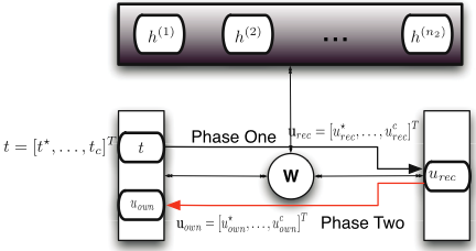
Having obtained 〈t⋆ , u⋆own 〉, the agent has now to decide on how to concede to t⋆ from tc. [Williams et al., 2011] adopted a linear concession strategy. However, such a scheme potentially omits a lot of relevant information about the opponent's model. To overcome such a shortcoming, this work uses the functional (i.e., learnt by the CRBM) manifold in order to determine the concession rate over time. First, a vector of equally spaced time intervals between t⋆ and tc is created. This vector is passed to the CRBM to predict a vector of relevant urec's (i.e., phase one in Figure 1). Having attained urec, the machine runs backwards, denoted by phase two in Figure 1, (i.e., CD with fixing the present layer and reconstructing on the input) to find the optimal utility to offer at the current time tc which is represented by uτ (see line 8 of Algorithm 1). It is clear that the concession rate follows the manifold created by the factored three-way weight tensor, and thus follows the surface of the learnt function. Adopting the above scheme, the agent potentially reaches 〈t⋆ , u⋆own 〉, which are used to attain u⋆rec such that the expected received utility can be maximized.
Given a utility (uτ ) to offer, the agent needs to validate whether the utility of the latest counter-offer is better than uτ and the (discounted) reservation value, or whether it had been already proposed earlier by the agent. If either of the conditions is met, the agent accepts this counter-offer and an agreement is reached as shown in line 10 of Algorithm 1. Otherwise, the proposed method constructs a new offer which has a utility of uτ . Furthermore, for negotiation efficiency, if uτ drops below the value of the best counter-offer, the agent chooses that best counter-offer as its next offer, because such a proposal tends to well satisfy the expectation of the opponent, which will then be inclined to accept it.
3.2 Transfer Mechanism
Knowledge transfer has been an essential integrated part of different machine learning algorithms. The idea behind transferring knowledge is that a target agents when faced by new and unknown tasks, may benefit from the knowledge gathered by other agents in different source tasks. Opponent modeling in complex negotiations is a tough challenge mainly due to the lack of enough information about the opponent. Transfer learning is a well suited potential solution for such a problem. In this paper and to the best of our knowledge, the first successful attempts for transferring between different negotiation tasks are reported.
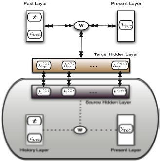
The overall transfer mechanism of TCRMB is shown in Figure 2. After learning in a source task, this knowledge is then mapped to the target. The mapping is manifested by the connections between the two tasks' hidden layers (Figure 2). This can be seen as an initialization of the target task machine using the source model. The intuition behind this idea is that even though the two tasks are different, they might have shared features. This relation is discovered using the weight connections between the hidden layers shown in Figure 2. To learn these weight connections contrastive divergence on the corresponding layers is performed. The weights are learnt such that the reconstruction error between these layers is minimized. It is worth pointing out that there is no need for the target hidden units to be same as these of the source. The following update rules for learning the weights are used:
where, WS→T is the weight connection between the source negotiation task, S, and the target task T , τ is the iteration step of contrastive divergence, α is the learning rate, 〈·〉 is the data distribution expectation and 〈·〉K is the reconstructed distribution after K-steps sampled through a Gibbs sampler from a Markov chain starting at the original data set.
When the weights are attained, an initialization of the target task hidden layer using the source knowledge is available. This is used at the start of the negotiation to propose offers for the new opponent. The scheme in which these propositions occur is the same as explained previously in the case of no transfer. When additional target information is gained, it is used to train the target CRBM as in the normal case. It is worth noting, that this proposed transfer method is not restricted to one source task. On the contrary, multiple source tasks are equally applicable. Furthermore, such a transfer scheme is different from just using the history of the agent. The transferred knowledge can arrive from any other task as long as this information is mapped correctly to suit the target. This mapping is performed using the CD algorithm as described above.
| Domain name | Number of issues | Number of values for each issue | Size of the outcome space |
|---|---|---|---|
| Energy | 8 | 5 | 390,625 |
| Travel | 7 | 4-8 | 188,160 |
| ADG | 6 | 5 | 15,625 |
| Music collection | 6 | 3-6 | 4,320 |
| Camera | 6 | 3-5 | 3,600 |
| Amsterdam party | 5 | 4-7 | 3,024 |
The difference between TCRMB and CRMB, as seen in line 6 of Algorithm 1, lies in the initialization procedure of the three-way weight tensor at the start of the negotiation. In case of TCRMB the initialization is performed using the transferred knowledge from the source task(s), while in CRMB this is done using the standard method, where the weights are sampled from a uniform Gaussian distribution with a mean and standard deviation determined by the designer.
4 Experiments and Results
The performance evaluation was done with GENIUS, which is also used as a competition platform for the negotiation competition (ANAC). The assessment quality under which the performance of the proposed method was evaluated is the competition results in the tournament format. The comparison between the transfer and the non-transfer case is thoroughly experimented, more details are given in Section 4.2. Furthermore, an empirical game theoretic evaluation is used to study the robustness of the proposed methods (Section 4.3).
4.1 Experiment setup
As most of the domains created for ANAC 2012 are not competitive enough, it is not hard for both parties to arrive at a win-win solution. To make the testing scenarios more challenging, six large outcome space domains are chosen. The characteristics of these domains are over-viewed in Table 1. Based on the above, a number of different random scenarios are generated to meet the following two inequities resulting in strictly conflicting preferences between two parties:
where V a j is the evaluation function of agent a for issue j, oj and o′j are different values for issue j.
where, wa i is the weight of issue j assigned to agent a.
Moreover, the discounting factor and the reservation value for each scenario are sampled from a uniform distribution, in the intervals [0.5, 1] and [0, 0.5], respectively. Furthermore, the selection of benchmarking agents is also a decisive factor to the quality of the evaluation. The eight finalists of the most recent competition (ANAC 2012) are therefore all included in the experiments. In addition the DragonAgent proposed in [Chen et al., 2013] is introduced as an extra benchmark. The experiment ran 10 times for every scenario to assure that the results are statistically significant. For the transfer setting, TCRMB is provided with no knowledge beforehand. It can rather use up to n previous sessions encountered acting on the same side/role (e.g., buyer or seller), with n being the total number of opponents. The number of intervals (i.e.,ζ) is set to 200. The hidden units in the CRBM and TCRBM are set to 20 and 30, respectively. A momentum of 0.9 as suggested in [Hinton, 2010] to increase the speed of learning is used. Furthermore, to avoid over-fitting, a weight-decay factor of 0.0002 (also used in [Hinton, 2010]) is adopted.
| Agent | Mean Score | Lower Bound | Upper Bound |
|---|---|---|---|
| TCRBMagent | 0.534 | 0.522 | 0.545 |
| CRBMagent | 0.485 | 0.471 | 0.499 |
| DragonAgent | 0.474 | 0.448 | 0.499 |
| AgentLG | 0.466 | 0.443 | 0.488 |
| BRAMAgent 2 | 0.465 | 0.443 | 0.487 |
| OMACagent | 0.456 | 0.438 | 0.472 |
| CUHKAgent | 0.447 | 0.425 | 0.467 |
| TheNegotiator | 0.429 | 0.415 | 0.442 |
| IAMhaggler2012 | 0.408 | 0.391 | 0.427 |
| AgentMR | 0.387 | 0.376 | 0.399 |
| Meta-Agent | 0.373 | 0.355 | 0.390 |
4.2 Competition results
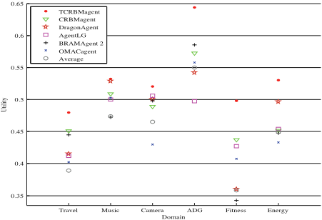
Figure 3 depicts the experimental results for the six domains, where the six top agents (according to the overall performance, see Table 2) and the mean score of all agents are shown, with self-play performance also considered.
Some interesting observations emerged from these outcomes. First, CRBMagent performs quite well against those strong agents from ANAC. It is generally ranked top three, and achieves on average 9.2% more than the mean performance of all participants. Then, relying on the framework of the former, TCRBMagent significantly outperforms other competitors by taking advantage of knowledge transfer. Clearly, it is the leading agent in all domains. Specifically, its performance is 19.2% higher than the mean score obtained by all agents across the domains. Moreover, it gains an improvement of 10.2% over CRBMagent, the second best agent in the experiments, while being more stable (i.e., experiencing less variance). This is due to the effect of knowledge transfer, where such a scheme biased the proposition of the agent towards better bidding process. Additionally, the performance of CUHKAgent, the winner of ANAC 2012, is surprisingly below the average. It is mainly because the strong agents like CRBMagent, TCRBMagent, and DragonAgent cause a considerable impact to CUHKAgent in such complex and high competitive domains, thereby suppressing its scores dramatically. It also explains why the ranking given in Table 2 is different from the final results of ANAC 2012.
4.3 The Empirical Game theoretic analysis
So far, the strategy performance was studied from the usual mean-scoring perspective. This, however, does not reveal information about the robustness of these strategies. To address robustness appropriately, empirical game theory (EGT) analysis [Jordan et al., 2007] is applied to the competition results. Here, we consider the best single-agent deviations as in [Williams et al., 2011], where there is an incentive for one agent to unilaterally change the strategy in order to statistically improve its own profit. The aim of using EGT is to search for pure Nash equilibria in which no agent has an incentive to deviate from its current strategy. The abbreviation for each strategy is indicated by the bold letter in Table 2. A profile (node) in the resulting EGT graph is defined by the mixture of strategies used by the players in a tournament. However, analysis of the 11-agent tournaments with the full combination of strategies is far too large to visualize. This is because (|p|+|s|-1 |p| ) = (21 11) = 352, 716 distinct nodes (where |p| is the number of players and |s| is the number of strategies) to represent in a graph using the technique. Due to space constraints, the analysis of 6-agent tournament in which each agent can choose one of the top six strategies reported in Table 2 are performed. For brevity reasons, we prune the graph to highlight some interesting features. To this end, the same pruning technique as in [Baarslag et al., 2013] was adopted. That is, only those nodes on the path leading to pure Nash equilibria, starting from an initial profile where all agent employ the same strategy or each agent use a different strategy are shown. Energy, as the largest domain, is selected as the target scenario. Under this EGT analysis, there exists only two pure Nash equilibria, represented by a thick border in Figure 4 as follows:
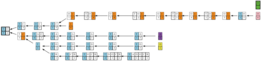
- All agents use the same strategy - BRAMagent 2.
- Four agents use TCRMB and two agents use CRMB.
The first Nash equilibrium is one of the initial states, where the self-play performance of BRAMagent 2 is pretty high so that no agent is motivated to deviate from the current state. No other profiles, however, are interested in switching to this profile. In contrast, the second equilibrium consisting of TCRMB and CRMB is of more interest, as it attracts all profiles except the first equilibrium state. In other words, for any non-Nash equilibrium strategy profile there exist a path of statistically significant deviations (i.e., strategy changes) that leads to this equilibrium. In the second equilibrium, there is no incentive for any agents to deviate from TCRMB to CRMB, as this will decrease their payoffs. The analysis reveals that the two proposed strategies are both robust.
5 Conclusions and FutureWork
In this paper two novel opponent modeling techniques, relying on deep learning methods, for highly competitive and complex negotiations are proposed. Based on these, two novel negotiation strategies are developed. Furthermore, to the best of our knowledge, the first successful results of transfer in negotiation scenarios are reported. Experimental results show both proposed strategies to be successful and robust.
The proposed method might suffer from a well-know transfer-related problem - Negative transfer. We speculate that TCRMB might avoid negative transfer in this context due to the highly informative and robust feature extraction scheme, as well as the hidden layer mapping. Nonetheless, a more thorough analysis, as well as possible quantifications of negative transfer are interesting directions for future work. Furthermore, the computational complexity of the proposed methods can still be reduced by adopting different sparse techniques frommachine learning.
Another interesting future direction is the extension of the proposed framework to concurrent negotiations. In such settings, the agent is negotiating against multiple opponents simultaneously. Transfer between these tasks can serve as a potential solution for optimizing the performance in each of the negotiation sessions.
@inproceedings{ijcai2013p21,
  title     = {Are There Any Nicely Structured Preference Profiles Nearby?},
  author    = {Bredereck, Robert and Chen, Jiehua and Woeginger, Gerhard J.},
  booktitle = {Proceedings of the Twenty-Third International Joint Conference on
               Artificial Intelligence, {IJCAI-13}},
  publisher = {AAAI Press / International Joint Conferences on Artificial Intelligence},
  editor    = {Francesca Rossi},
  pages     = {62--67},
  year      = {2013},
  month     = {8},
  url       = {https://ijcai.org/proceedings/2013/21},
}
TY - CPAPER TI - Are There Any Nicely Structured Preference Profiles Nearby? AU - Bredereck, Robert AU - Chen, Jiehua AU - Woeginger, Gerhard J. T2 - Proceedings of the Twenty-Third International Joint Conference on Artificial Intelligence, IJCAI-13 PB - AAAI Press / International Joint Conferences on Artificial Intelligence PY - 2013 SP - 62 EP - 67 UR - https://ijcai.org/proceedings/2013/21 ER -Copied
Machine-readable versions of this paper, for tools and AI agents:





