Maximal Recursive Rule: A New Social Decision Scheme

1 Introduction

In a seminal paper, Gary Becker [1968] presented a compelling economic treatment of crime and punishment. He demonstrated that effective law enforcement involves optimal resource allocation to prevent and detect violations, coupled with appropriate punishments for offenders. He described how to optimize resource allocation by balancing the societal cost of crime and the cost incurred by prevention, detection and punishment schemes. While Becker focused on crime and punishment in society, similar economic considerations guide enforcement of a wide range of policies. In this paper, we study effective enforcement mechanisms for this broader set of policies. Our study differs from Becker's in two significant ways-our model accounts for strategic interaction between the enforcer (or defender) and the adversary; and we design efficient algorithms for computing the optimal resource allocation for prevention or detection measures as well as punishments. At the same time, our model is significantly less nuanced than Becker's, thus enabling the algorithmic development and raising interesting questions for further work.

∗This work was partially supported by ARO contract DAAD1902-1-0389, NSF TRUST Center, AFOSR MURI Collaborative Policies and Assured Information Sharing, HHS Grant no. HHS 90TR0003/01 and NSF CCF-1215883. J. Blocki and A. Sinha were also partially supported by an NSF Graduate Fellowship and a CMU CIT Bertucci Fellowship, respectively. The views and conclusions contained in this document are those of the authors only.

A motivating application for our work is auditing, which typically involves detection and punishment of policy violators. In particular, enforcement of privacy laws and policies in modern organizations that hold large volumes of personal information (e.g., hospitals, banks, and Web services providers like Google and Facebook) relies heavily on internal audit mechanisms. Audits are also common in the financial sector (e.g., to identify fraudulent transactions), in internal revenue services (e.g., to detect tax evasion), and in traditional law enforcement (e.g., to catch speed limit violators).

The audit process is an interaction between two agents: a defender (auditor) and an adversary (auditee). As an example, consider a hospital (defender) auditing its employee (adversary) to detect privacy violations committed by the employee when accessing personal health records of patients. While privacy violations are costly for the hospital as they result in reputation loss and require expensive measures (such as privacy breach notifications), audit inspections also cost money (e.g., the cost of the human auditor involved in the investigation). Moreover, the number and type of privacy violations depend on the actions of the rational auditee-employees commit violations that benefit them.

1.1 Our Model

We model the audit process as a game between a defender (e.g, a hospital) and an adversary (e.g., an employee). The defender audits a given set of targets (e.g., health record accesses) and the adversary chooses a target to attack. The defender's action space in the audit game includes two components. First, the allocation of its inspection resources to targets; this component also exists in a standard model of security games [Tambe, 2011]. Second, we introduce a continuous punishment rate parameter that the defender employs to deter the adversary from committing violations. However, punishments are not free and the defender incurs a cost for choosing a high punishment level. For instance, a negative work environment in a hospital with high fines for violations can lead to a loss of productivity (see [Becker, 1968] for a similar account of the cost of punishment). The adversary's utility includes the benefit from committing violations and the loss from being punished if caught by the defender. Our model is parametric in the utility functions. Thus, depending on the application, we can instantiate the model to either allocate resources for detecting violations or preventing them. This generality implies that our model can be used to study all the applications previously described in the security games literature [Tambe, 2011].

To analyze the audit game, we use the Stackelberg equilibrium solution concept [von Stackelberg, 1934] in which the defender commits to a strategy, and the adversary plays an optimal response to that strategy. This concept captures situations in which the adversary learns the defender's audit strategy through surveillance or the defender publishes its audit algorithm. In addition to yielding a better payoff for the defender than any Nash equilibrium, the Stackelberg equilibrium makes the choice for the adversary simple, which leads to a more predictable outcome of the game. Furthermore, this equilibrium concept respects the computer security principle of avoiding "security through obscurity"- audit mechanisms like cryptographic algorithms should provide security despite being publicly known.

1.2 Our Results

Our approach to computing the Stackelberg equilibrium is based on the multiple LPs technique of Conitzer and Sandholm [2006]. However, due to the effect of the punishment rate on the adversary's utility, the optimization problem in audit games has quadratic non-convex constraints. The nonconvexity does not permit the use of any convex optimization methods, and in general efficient solutions for a broad class of non-convex problems are not known [Neumaier, 2004].

However, we demonstrate that we can efficiently obtain an additive approximation to our problem. Specifically, we present an additive fully polynomial time approximation scheme (FPTAS) to solve the audit game optimization problem. Our algorithm provides a K-bit precise output in time polynomial in K. Also, if the solution is rational, our algorithm provides an exact solution in polynomial time. In general, the exact solution may be irrational and may not be representable in a finite amount of time.

1.3 RelatedWork

Our audit game model is closely related to security games [Tambe, 2011]. There are many papers (see, e.g., [Korzhyk et al., 2010; Pita et al., 2011; 2008]) on security games, and as our model adds the additional continuous punishment parameter, all the variations presented in these papers can be studied in the context of audit games (see Section 4). However, the audit game solution is technically more challenging as it involves non-convex constraints.

An extensive body of work on auditing focuses on analyzing logs for detecting and explaining violations using techniques based on logic [Vaughan et al., 2008; Garg et al., 2011] and machine learning [Zheng et al., 2006; Bodik et al., 2010]. In contrast, very few papers study economic considerations in auditing strategic adversaries. Our work is inspired in part by the model proposed in one such paper [Blocki et al., 2012], which also takes the point of view of commitment and Stackelberg equilibria to study auditing. However, the emphasis in that work is on developing a detailed model and using it to predict observed audit practices in industry and the effect of public policy interventions on auditing practices. They do not present efficient algorithms for computing the optimal audit strategy. In contrast, we work with a more general and simpler model and present an efficient algorithm for computing an approximately optimal audit strategy. Furthermore, since our model is related to the security game model, it opens up the possibility to leverage existing algorithms for that model and apply the results to the interesting applications explored with security games.

Zhao and Johnson [2008] model a specific audit strategy: agents are permitted to violate an access control policy at their discretion (e.g., in an emergency situation in a hospital), but these actions are audited. They manually analyze specific utility functions and obtain closed-form solutions for the audit strategy that results in a Stackelberg equilibrium. In contrast, our results apply to any utility function and we present an efficient algorithm for computing the audit strategy.

2 The Audit Game Model

The audit game features two players: the defender (D), and the adversary (A). The defender wants to audit n targets t1, . . . , tn, but has limited resources which allow for auditing only one of the n targets. Thus, a pure action of the defender is to choose which target to audit. A randomized strategy is a vector of probabilities p1, . . . , pn of each target being audited. The adversary attacks one target such that given the defender's strategy the adversary's choice of violation is the best response.

Let the utility of the defender be U aD (ti) when audited target ti was found to be attacked, and U uD (ti) when unaudited target ti was found to be attacked. The attacks (violation) on unaudited targets are discovered by an external source (e.g. government, investigative journalists,...). Similarly, define the utility of the attacker as U aA(ti) when the attacked target ti is audited, and U uA(ti) when attacked target ti is not audited, excluding any punishment imposed by the defender. Attacks discovered externally are costly for the defender, thus, U aD (ti) > U uD (ti). Similarly, attacks not discovered by internal audits are more beneficial to the attacker, and U uA(ti) > U aA(ti).

The model presented so far is identical to security games with singleton and homogeneous schedules, and a single resource [Korzhyk et al., 2010]. The additional component in audit games is punishment. The defender chooses a punishment "rate" x ∈ [0, 1] such that if auditing detects an attack, the attacker is fined an amount x. However, punishment is not free-the defender incurs a cost for punishing, e.g., for creating a fearful environment. For ease of exposition, we model this cost as a linear function ax, where a > 0; however, our results directly extend to any cost function polynomial in x. Assuming x ∈ [0, 1] is also without loss of generality as utilities can be scaled to be comparable to x. We do assume the punishment rate is fixed and deterministic; this is only natural as it must correspond to a consistent policy.

We can now define the full utility functions. Given probabilities p1, . . . , pn of each target being audited, the utility of the defender when target t∗ is attacked is

The defender pays a fixed cost ax regardless of the outcome. However, the attacker suffers the punishment x only when attacking an audited target. Thus, in the same scenario, the utility of the attacker when target t∗ is attacked is

Equilibrium. The Stackelberg equilibrium solution involves a commitment by the defender to a strategy (with a possibly randomized allocation of the resource), followed by the best response of the adversary. The mathematical problem involves solving multiple optimization problems, one each for the case when attacking t∗ is in fact the best response of the adversary. Thus, assuming t∗ is the best response of the adversary, the ∗th optimization problem P∗ in audit games is

The first constraint verifies that attacking t∗ is indeed a best response. The auditor then solves the n problems P1, . . . , Pn (which correspond to the cases where the best response is t1, . . . , tn, respectively), and chooses the best solution among all these solutions to obtain the final strategy to be used for auditing. This is a generalization of the multiple LPs approach of Conitzer and Sandholm [2006].

Inputs. The inputs to the above problem are specified in Kbit precision. Thus, the total length of all inputs is O(nK).

3 Computing an Audit Strategy

Because the indices of the set of targets can be arbitrarily permuted, without loss of generality we focus on one optimization problem Pn (∗ = n) from the multiple optimization problems presented in Section 2. The problem has quadratic and non-convex constraints. The non-convexity can be readily checked by writing the constraints in matrix form, with a symmetric matrix for the quadratic terms; this quadratic-term matrix is indefinite.

However, for a fixed x, the induced problem is a linear programming problem. It is therefore tempting to attempt a binary search over values of x. This na¨ıve approach does not work, because the solution may not be single-peaked in the values of x, and hence choosing the right starting point for the binary search is a difficult problem. Another na¨ıve approach is to discretize the interval [0, 1] into steps of ϵ′ , solve the resultant LP for the 1/ϵ′ many discrete values of x, and then choose the best solution. As an LP can be solved in polynomial time, the running time of this approach is polynomial in 1/ϵ′ , but the approximation factor is at least aϵ′ (due to the ax in the objective). Since a can be as large as 2K , getting an ϵ-approximation requires ϵ′ to be 2-K ϵ, which makes the running time exponential in K. Thus, this scheme cannot yield an FPTAS.

3.1 High-Level Overview

Fortunately, the problem Pn has another property that allows for efficient methods. Let us rewrite Pn in a more compact form. Let ∆D,i = U aD (ti) - U uD (ti), ∆i = U uA(ti) - U aA(ti) and δi,j = U uA(ti)-U uA(tj). ∆D,i and ∆i are always positive, and Pn reduces to:

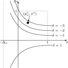
The main observation that allows for polynomial time approximation is that, at the optimal solution point, the quadratic constraints can be partitioned into a) those that are tight, and b) those in which the probability variables pi are zero (Lemma 1). Each quadratic constraint corresponding to pi can be characterized by the curve pn(x +∆n) + δi,n = 0. The quadratic constraints are thus parallel hyperbolic curves on the (pn, x) plane; see Figure 1 for an illustration. The optimal values pon , xo partition the constraints (equivalently, the curves): the constraints lying below the optimal value are tight, and in the constraints above the optimal value the probability variable pi is zero (Lemma 2). The partitioning allows a linear number of iterations in the search for the solution, with each iteration assuming that the optimal solution lies between adjacent curves and then solving the sub-problem with equality quadratic constraints.

Next, we reduce the problem with equality quadratic constraints to a problem with two variables, exploiting the nature of the constraints themselves, along with the fact that the objective has only two variables. The two-variable problem can be further reduced to a single-variable objective using an equality constraint, and elementary calculus then reduces the problem to finding the roots of a polynomial. Finally, we use known results to find approximate values of irrational roots.

3.2 Algorithm andMain Result

The main result of our paper is the following theorem:

Theorem 1. Problem Pn can be approximated to an additive ϵ in time O(n5K + n4 log( 1ϵ )) using the splitting circle method [Sch¨onhage, 1982] for approximating roots.

Remark The technique of Lenstra et al. [1982] can be used to exactly compute rational roots. Employing it in conjunction with the splitting circle method yields a time bound O(max{n13K3 , n5K +n4 log(1/ϵ)}). Also, this technique finds an exact optimal solution if the solution is rational.

Before presenting our algorithm we state two results about the optimization problem Pn that motivate the algorithm and are also used in the correctness analysis. All missing proofs in this paper are present in the full version of the paper. 1

Lemma 1. Let pon , xo be the optimal solution. Assume xo > 0 and pon < 1. Then, at pon , xo , for all i ̸= n, either pi = 0 or pon (xo +∆n) + δi,n = pi(xo +∆i), i.e., the ith quadratic constraint is tight.

Lemma 2. Assume xo > 0 and pon < 1. Let pon (xo +∆n) + δ = 0. If for some i, δi,n < δ then pi = 0. If for some i, δi,n > δ then pon (xo +∆n)+δi,n = pi(xo +∆i). If for some i, δi,n = δ then pi = 0 and pon (xo+∆n)+δi,n = pi(xo+∆i).

Proof. The quadratic constraint for pi is pon (xo+∆n)+δi,n ≤ pi(xo +∆i). By Lemma 1, either pi = 0 or the constraint is tight. If pon (xo +∆n) + δi,n < 0, then, since pi ≥ 0 and xo +∆i ≥ 0, the constraint cannot be tight. Hence, pi = 0. If pon (xo +∆n)+δi,n > 0, then, pi ̸= 0 or else with pi = 0 the constraint is not satisfied. Hence the constraint is tight. The last case with pon (xo + ∆n) + δi,n = 0 is trivial.

From Lemma 2, if pon , xo lies in the region between the adjacent hyperbolas given by pon (xo + ∆n) + δi,n = 0 and pon (xo + ∆n) + δj,n = 0 (and 0 < xo ≤ 1 and 0 ≤ pon < 1), then δi,n ≤ 0 and pi ≥ 0 and for the kth quadratic constraint with δk,n < δi,n, pk = 0 and for the j th quadratic constraint with δj,n > δi,n, pj ̸= 0 and the constraint is tight.

These insights lead to Algorithm 1. After handling the case of x = 0 and pn = 1 separately, the algorithm sorts the δ's to get δ(1),n, . . . , δ(n-1),n in ascending order. Then, it iterates over the sorted δ's until a non-negative δ is reached, assuming the corresponding pi's to be zero and the other quadratic constraints to be equalities, and using the subroutine EQ OPT to solve the induced sub-problem. For ease of exposition we assume δ's to be distinct, but the extension to repeated δ's is quite natural and does not require any new results. The subproblem for the ith iteration is given by the problem Qn,i:

1 http://arxiv.org/abs/1303.0356

Algorithm 1: APX SOLVE(ϵ, Pn)

l ← prec(ϵ, n, K), where prec is defined after Lemma 7 Sort δ's in ascending order to get δ(1),n, . . . , δ(n-1),n, with corresponding variables p(1), . . . , p(n-1) and quadratic constraints C(1), . . . , C(n-1) Solve the LP problem for the two cases when x = 0 and pn = 1 respectively. Let the solution be S0 , p0(1) , . . . , p0(n-1) , p0n , x0 and S-1 , p-1 (1) , . . . , p-1 (n-1) , p-1 n , x-1 respectively. for i ← 1 to n - 1 do if δ(i),n ≤ 0 ∨ (δ(i),n > 0 ∧ δ(i-1),n < 0) then p(j) ← 0 for j < i. Set constraints C(i), . . . , C(n-1) to be equalities. Si , pi(1) , . . . , pi(n-1) , pin , xi ← EQ OPT(i, l) elseSi ← -∞ f ← argmaxi{S-1 , S0 , S1 , . . . , Si , . . . , Sn-1} pf1 , . . . , pfn-1 ← Unsort pf(1) , . . . , pf(n-1) return pf1 , . . . , pfn , xf

The best (maximum) solution from all the sub-problems (including x = 0 and pn = 1) is chosen as the final answer.

Lemma 3. Assuming EQ OPT produces an ϵ-additive approximate objective value, Algorithm 1 finds an ϵ-additive approximate objective of optimization problem Pn.

EQ OPT solves a two-variable problem Rn,i instead of Qn,i. The problemRn,i is defined as follows:

The following result justifies solving Rn,i instead of Qn,i.

Lemma 4. Qn,i and Rn,i are equivalent for all i.

Proof. Since the objectives of both problems are identical, we prove that the feasible regions for the variables in the objective (pn, x) are identical. Assume pn, x, p(i), . . . , p(n-1) is feasible in Qn,i. The first two constraints are the same in Qn,i and Rn,i. Divide each equality quadratic constraint corresponding to non-zero p(j) by x + ∆(j). Add all such constraints to get:

Algorithm 2: EQ OPT(i, l)

Then, since ∑k:1≤k≤i p(k) = 1 - pn we get

The last two constraints are the same in Qn,i and Rn,i. Next, assume pn, x is feasible in Rn,i. Choose p(j) = pn ( x+∆n x+∆(j) ) + δ(j),n x+∆(j) . Since pn(x+∆n)+δ(i),n ≥ 0, we have p(i) ≥ 0, and since pn(x + ∆n) + δ(j),n > 0 for j > i (δ's are distinct) we have p(j) > 0. Also,

which by the third constraint of Rn,i is 1-pn, thus, p(j) ≤ 1. Thus, pn, x, p(i), . . . , p(n-1) is feasible in Qn,i.

The equality constraint in Rn,i, which forms a curve Ki, allows substituting pn with a function Fi(x) of the form f(x)/g(x). Then, the steps in EQ OPT involve taking the derivative of the objective f(x)/g(x) and finding those roots of the derivative that ensure that x and pn satisfy all the constraints. The points with zero derivative are however local maxima only. To find the global maxima, other values of x of interest are where the curve Ki intersects the closed boundary of the region defined by the constraints. Only the closed boundaries are of interest, as maxima (rather suprema) attained on open boundaries are limit points that are not contained in the constraint region. However, such points are covered in the other optimization problems, as shown below.

The limit point on the open boundary pn(x + ∆n) + δ(i-1),n < 0 is given by the roots of Fi(x) + δ(i-1),n x+∆n . This point is the same as the point considered on the closed boundary pn(x + ∆n) + δ(i-1),n ≥ 0 in problem Rn,i-1 given by roots of Fi-1(x) + δ(i-1),n x+∆n , since Fi-1(x) = Fi(x) when pn(x +∆n) + δ(i-1),n = 0. Also, the other cases (x = 0 and pn = 1) are covered by the LP solved at the beginning of Algorithm 1.

The closed boundary in Rn,i are obtained from the constraint pn(x +∆n) + δ(i),n ≥ 0, 0 ≤ pn and x ≤ 1. The value x of the intersection of pn(x + ∆n) + δ(i),n = 0 and Ki is given by the roots of Fi(x) + δ(i),n x+∆n = 0. The value x of the intersection of pn = 0 and Ki is given by roots of Fi(x) = 0. The value x of the intersection of x = 1 and Ki is simply x = 1. Additionally, as checked in EQ OPT, all these intersection points must lie with the constraint regions defined in Qn,i.

The optimal x is then the value among all the points of interest stated above that yields the maximum value for f(x) g(x) . Algorithm 2 describes EQ OPT, which employs a root finding subroutine ROOTS. Algorithm 2 also takes care of approximate results returned by the ROOTS. As a result of the 2-l approximation in the value of x, the computed x and pn can lie outside the constraint region when the actual x and pn are very near the boundary of the region. Thus, we check for containment in the constraint region for points x ± 2-l and accept the point if the check passes.

3.3 Analysis

Before analyzing the algorithm's approximation guarantee we need a few results that we state below.

Lemma 5. The maximum bit precision of any coefficient of the input polynomials to ROOTS is 2n(K + 1.5) + log(n).

Proof. The max. bit precision is obtained in g(x)f ′ (x) - f(x)g′ (x). Consider the worst case when i = 1. Then, f(x) is of degree n and g(x) of degree n - 1. Therefore, the bit precision of f(x) and g(x) is upper bounded by nK + log(( n n/2)), where nK comes from multiplying n Kbit numbers and log(( n n/2)) arises from the maximum number of terms summed in forming any coefficient. Thus, using the fact that ( n n/2) ≤ (2e)n/2 the upper bound is approximately n(K+1.5). We conclude that the bit precision of g(x)f ′ (x)- f(x)g′ (x) is upper bounded by 2n(K + 1.5) + log(n).

We can now use Cauchy's result on bounds on root of polynomials to obtain a lower bound for x. Cauchy's bound states that given a polynomial anxn + . . . + a0, any root x satisfies

Using Lemma 5, it can be concluded that any positive root of the polynomial input to ROOTS satisfies x > 2-4n(K+1.5)-2 log(n)-1 = B. The following lemma bounds the additive approximation error.

Lemma 6. Assume that x > B and |x - x′ | ≤ ϵ < B/2 then for any index i in Algorithm 2 we have |Fi(x) -Fi(x′ )| ≤ ϵΨ, where Ψ is of order O(n2(8n(K+1.5)+4 log(n)+K ).

We are finally ready to establish the approximation guarantee of our algorithm.

Lemma 7. Algorithm 1 solves problem Pn with additive approximation term ϵ if

Also, as log( ∆D,nΨ+a ϵ ) = O(nK + log( 1ϵ )), l is of order O(nK + log( 1ϵ )).

Proof. Let x denote the optimal punishment level and let x′ denote the corresponding approximation returned by EQ OPT. If ROOTS is called by EQ OPT with accuracy parameter l then |x′ -x| ≤ 2 · 2-l . The additional factor of 2 arises due to the boundary check in EQ OPT. Let p′n denote our approximation to the optimal inspection rate pn. If we set l > 1 + log( ∆D,nΨ+a ϵ ) and apply Lemma 6 then

The other term in the max above arises from the condition 2 · 2-l < B/2 in Lemma 6.

As the upper bound on ψ is only in terms of n and K, we can express l as a function of ϵ, n and K: l = prec(ϵ, n,K).

We still need to analyze the running time of the algorithm. For ease of notation, we use O(n) as the time of multiplication of n bit numbers obtained on a pointer based Turing machine. The same on a normal Turing machine is O(n log n log log n), which also results in an overall polynomial running time. Next, we briefly discuss the known algorithms that we use and their corresponding running-time guarantees. Linear programming can be done in polynomial time using Karmakar's algorithm [Karmarkar, 1984] with a time bound of O(n3.5L), where L is the length of all inputs.

The splitting circle scheme to find roots of a polynomial combines many varied techniques. The core of the algorithm yields linear polynomials Li = aix+bi (a, b can be complex) such that |P - ∏i Li| < 2-s . The norm |.| considered is the sum of absolute values of the coefficient. The running time of the algorithm is O(n3 log n + n2 s) in a pointer based Turing machine. By choosing s = θ(nl) and choosing the real part of those complex roots that have imaginary value less than 2-l , it is possible to obtain approximations to the real roots of the polynomial with l bit precision in time O(n3 log n+n3 l).

The above method may yield real values that lie near complex roots. However, such values will be eliminated in taking the maximum of the objective over all real roots, if they do not lie near a real root.

With these properties, we can state the following lemma.

Lemma 8. The running time of Algorithm 1 with input approximation parameter ϵ and inputs of K bit precision is bounded by O(n5K + n4 log( 1ϵ )) .

Proof. We use T (n,K, ϵ), E (n, l), R(n, l), and H(n, l) respectively to denote the running times of Algorithm 1, EQ OPT, ROOTS and Horner's method [Horner, 1819] for evaluating a degree n polynomial with ℓ bits of precision. On a pointer-based machine we have R(n, l) = O (n3 log n + n3 l) and H(n, l) = O (n2 l). EQ OPT makes 3 calls to ROOTS, and evaluates one polynomial so we have

From Lemma 7 we get l = O (nK + n log ( 1ϵ )). As the linear programs can be computed in O(n4.5K) and Algorithm 1 calls EQ OPT at most n times T (n, K, ϵ) is bounded by

4 Discussion

We have introduced a novel model of audit games. Our model augments the simplest model of security games with a punishment parameter. However, the security game framework is in general much more expressive. The model [Kiekintveld et al., 2009] includes a defender that controls multiple security resources, where each resource can be assigned to one of several schedules, which are subsets of targets. This notion of schedules also applies to audit games, e.g., in organizations managers (resources) are often required to audit actions of their direct employees. Other generalizations of security games include an adversary that attacks multiple targets [Korzhyk et al., 2011], and a defender with a budget [Bhattacharya et al., 2011]. These characteristics as well as the repeated nature of audits raise interesting modeling questions some of which have been studied in our prior work on audit games [Blocki et al., 2012]. The associated algorithmic questions are another exciting direction for future work.

Ultimately, we view our work as a first step toward a computationally feasible model of audit games. We envision a vigorous interaction between AI researchers and security and privacy researchers, which can quickly lead to deployed applications, especially given the encouraging precedent set by the deployment of security games algorithms [Tambe, 2011].