Learning from Polyhedral Sets

1 Introduction

Linear systems of inequalities over real numbers are basic tools for representing and reasoning over polyhedral sets. They have been extensively adopted in several fields of artificial intelligence, including geometric reasoning [Arnon, 1988], constraint (logic) programming [Jaffar et al., 1992], robot motion planning [Hwang and Ahuja, 1992], computer vision [Baumgart, 1975], resource planning [Wolfman and Weld, 2001], pattern recognition and classification [Smaoui et al., 2009], expert systems [McBride and O'Leary, 1993].

Suppose we are given two sample linear systems:

whose solutions, i.e., their polyhedra, describe a 2 × 3 and a 3 × 2 rectangle respectively. What should be a generalization of the two samples? Namely, how would we describe a class of polyhedra including the two rectangles above, and not much more? We call this kind of inferences the learning from polyhedral sets problem. The language for representing generalizations is a minimalist extension of the expressive power of linear systems admitting parameters among the constant terms. For instance, 0 ≤ x ≤ a, 0 ≤ y ≤ b is a parameterized linear system, where a and b are parameters and x and y are variables. The intended meaning of a parameterized linear system [Gal, 1995; Kvasnica, 2009; Pistikopoulos et al., 2007] is a class of polyhedra over variables, each obtained by instantiating the parameters. The parameterized system above then includes as special cases the polyhedra of the two sample systems (fixing a = 2, b = 3 and a = 3, b = 2 respectively). However, the system is too general, since there are rectangles a × b that are not proper generalizations of the two systems. The parameterized system 0 ≤ x ≤ a, 0 ≤ y ≤ b, 2 ≤ a ≤ 3, 2 ≤ b ≤ 3 describes a smaller class of polyhedra, still including the two samples, consisting of rectangles a × b whose sides are of size between 2 and 3. An even smaller generalization is 0 ≤ x ≤ a, 0 ≤ y ≤ 5 - a, 2 ≤ a ≤ 3: the two sample polyhedra are obtained for a = 2 and a = 3 respectively. This generalization captures the "convex" dependence between the sides of the two sample rectangles. When the length of the x side passes from 2 to 3, then the length of the y side linearly passes from 3 to 2 (due to the bound 5 - a). The method we devise for learning generalizations from example polyhedral sets leads to this last parameterized system.

This paper is organized as follows. We recall basic notation in Section 2. Parameterized linear systems are described in Section 3. The learning problem is introduced and investigated in Section 4. Finally, we summarize our contribution.

2 Background

We adhere to standard notation of linear algebra [Schrijver, 1987]. R is the set of real numbers. Small bold letters (a, b, . . . ) denote column vectors, while capital bold letters (A, B, . . . ) denote matrices. 0 is a column vector with all elements equal to 0. The transposed vector of a is denoted by aT . The inner product is denoted by aT · b. We write A · x ≤ b for a system of linear inequalities over the variables in x, also called a linear system. Given two linear systems P and S, we write P, S to denote the linear system consisting of the inequalities appearing in P or in S. A polyhedron is the set of solution points of a linear system: Sol(A · x ≤ b) = {x0 ∈ R|x| | A · x0 ≤ b}. Polyhedra are convex sets. The homogeneous version of a linear system H(A·x ≤ b) = A·x ≤ 0 is the linear system where constant terms are replaced by 0's. The characteristic cone, or simply the cone, of a non-empty polyhedron Sol(P) is Sol(H(P)). A polytope is the convex hull ConvexHull(x1, . . . , xn) of a finite set of vectors x1, . . . , xn, called vertices, namely the smallest polyhedron containing all the vectors. With some overload of terminology, by stating that a system P is the convex hull of x1, . . . , xn, we actually mean that Sol(P) = ConvexHull(x1, . . . , xn). A polyhedron is a polytope iff it is upper and lower bounded along every dimension.

Consider two linear systems P1 : A · x ≤ b and P2 : C · x ≤ d. The entailment problem consists of checking whether every solution of P1 is a solution of P2, namely whether Sol(P1) ⊆ Sol(P2) or, alternatively, whether the first-order formula ∀x [P1 → P2] holds over the domain of the reals. If this is the case, we say that P1 entails P2. Deciding whether P1 entails P2, can be solved in polynomial time [Subramani, 2009]. It suffices to show that for every inequality cT · x ≤ di in P2, the following linear programming problem is either infeasible or its solution is bounded by di:

The conclusion follows since linear programming problems are solvable in polynomial time [Khachiyan, 1979] and there is a finite number of inequalities in P2. As a consequence, checking equality of polyhedra, namely whether Sol(P1) = Sol(P2), is also a problem in P, since it reduces to show that P1 entails P2 and vice-versa.

3 Parameterized Linear Systems

A parameterized linear system over the reals is a system of linear inequalities A · x ≤ b+M· r where variables in r are parameters. The intended meaning of a parameterized linear system is a collection of linear systems over variables in x, each obtained by instantiating the parameters r. The notion of parameterized polyhedra from [Loechner and Wilde, 1997] models the solutions of parameterized linear systems.

Definition 3.1 A parameterized polyhedron is a collection of polyhedra defined by fixing the value of parameters in a parameterized linear system: Sol(A · x ≤ b+M· r, r0) = {x0 ∈ R|x| | A · x0 ≤ b+M· r0}, where r0 ∈ R|r| is an instance of the parameters r.

The Sol() function now returns the set of solution points of a parameterized linear system for a specific assignment to parameters. Let us introduce a notation for the class of polyhedra defined by a parameterized linear system. We define [[A · x ≤ b +M · r]] as

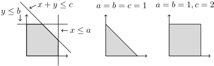
Example 3.1 Figure 1 shows the parameterized linear system 0 ≤ x ≤ a, 0 ≤ y ≤ b, x + y ≤ c, where x, y are variables and a, b, c are parameters. Several types of polytopes can be obtained as special cases: rectangled-isosceles triangles by setting a, b, c to a same value (1 in the figure), squares by setting a, b to a same value v, and c ≥ 2v (v = 1 in the figure), rectangles by setting c ≥ a + b, and, in addition, some classes of right trapezoids, and some classes of irregular pentagons.

The expressive power of parameterized linear systems is limited by the fact that parameters can only appear in constant terms. As an example, the class of rectangled triangles cannot be defined because it requires inequalities with parameters appearing as coefficients of variables. For instance, the inequality dx+y ≤ c in place of x+y ≤ c in Figure 1 would allow for defining hypotenuses with any angle of inclination.

The notion of entailment has been extended to parameterized linear system in [Eirinakis et al., 2012]. Let us recall here the case of two systems with disjoint parameters.

Definition 3.2 P1 = A1 · x ≤ b1 +M1 · r entails P2 = A2 · x ≤ b2 +M2 · s, with r ∩ s = ∅, if for every r0 ∈ ℜ|r| there exists s0 ∈ ℜ|s| such that Sol(P1, r0) ⊆ Sol(P2, s0).

Intuitively, P1 entails P2 if every parameter instance of P1 entails some parameter instance of P2. Notice that entailment is transitive. Finally, the homogeneous version of a parameterized linear system A · x ≤ b +M · r is defined as H(A · x ≤ b +M · r) = A · x ≤ 0. This conservatively extends the definition of H() for non-parameterized systems.

4 The Learning Problem

4.1 Problem Statement

Intuitively, learning from a collection of polyhedral sets consists of computing a parameterized linear system P whose class includes given sets Sol(Ai · x ≤ bi), with i = 1 . . . N.

Definition 4.1 (Generalization) A parameterized linear system P is a generalization of the linear systems P1, . . . , PN, if for i = 1 . . .N, there exists ri s.t. Sol(P, ri) = Sol(Pi).

In symbols, the definition can be re-stated by requiring:

A basic question is whether there exists P such that [[P]] is exactly the set {Sol(Pi) | i = 1 . . .N}. The answer is positive when such a set is a singleton or consists of an empty and a non-empty polyhedron. 1 In general, the answer is negative.

Lemma 4.1 Let P be a generalization of P1, . . . , Pn. Assume that there exist i, j such that ∅ ̸= Sol(Pi) ̸= Sol(Pj) ̸= ∅. Then [[P]] ⊃ {Sol(Pi) | i = 1 . . .N}.

Proof. For some ri ̸= rj, we have Sol(P, ri) = Sol(Pi) and Sol(P, rj) = Sol(Pj). Let xi ∈ Sol(P, ri) ̸= ∅ and xj ∈ Sol(P, rj) ̸= ∅. We have that (xi ri) and (xj rj) are solutions of the non-parameterized linear system P considered over the space of variables plus parameters. Since Sol(P) is a convex set, for every λ ∈ [0, 1], we have that λ(xi ri) + (1 - λ)(xj rj) is a solution of P, which implies Sol(P, (λri + (1 - λ)rj)) ̸= ∅. Since ri ̸= rj, this implies that [[P]] is infinite, hence it strictly includes the finite set {Sol(Pi) | i = 1 . . .N}. □

This motivates the introduction of the learning problem from polyhedral sets as a search problem among the generalizations of given polyhedral sets.

Definition 4.2 (Learning problem) Given N linear systems Pi = Ai · x ≤ bi such that Sol(Pi) ̸= ∅, with i = 1 . . .N, the learning problem consists of computing (if it exists) a generalization P of P1, . . . , PN.

1 For singletons, fix P to any Pi. In the latter case, by fixing P to (Pi, a = 0), where Sol(Pi) ̸= ∅ and a is a fresh parameter, it turns out [[P]] = {Sol(Pi), ∅}.

The assumption that the polyhedral sets Sol(Pi) are nonempty is not a loss of generality. We can always restrict the search to generalizations of non-empty sets, and then, from one of such generalizations, compute a generalization that includes the empty set.

Lemma 4.2 Let P be a generalization of P1, . . . , PN, with Sol(P, ri) = Sol(Pi), for i = 1 . . . N.

By defining S as the convex hull of r1, . . . , rn, we have that P ′ = P, S is a generalization of P1, . . . , PN such that Sol(P ′ , ri) = Sol(Pi), for i = 1 . . .N, and such that for some r0, Sol(P ′ , r0) = ∅.

Proof. Since ri ∈ Sol(S), we readily have Sol(P ′ , ri) = Sol(P, ri) = Sol(Pi). Since Sol(S) is a polytope, hence bounded, there exists r0 ̸∈ Sol(S). For such an r0 we have Sol(P ′ , r0) = ∅. □

Observe that a generalization may not always exist.

Example 4.1 Consider the linear systems x ≤ 0 and y ≤ 0. Any generalization P must impose an upper bound on both x (to cover the first system) and y (to cover the second system). For every parameter instance r0, there is then an upper bound for both x and y in Sol(P, r0). Since x ≤ 0 imposes no upper bound on y, we have Sol(P, r0) ̸= Sol(x ≤ 0) for every r0.

The intuition underlying the example is formalized next in a necessary condition for the existence of solutions to a learning problem. Later on, it will be shown to be also sufficient.

Lemma 4.3 If there exists a generalization of Pi = Ai · x ≤ bi, with i = 1 . . . N, then all Pi's have the same cone, i.e., for i, j = 1 . . . N we have Sol(Ai · x ≤ 0) = Sol(Aj · x ≤ 0).

Proof. Assume P = C · x ≤ d +M · r is a generalization, and Sol(Ai · x ≤ bi) = Sol(P, ri) = Sol(C · x ≤ d + M · ri), for i = 1 . . .N. By the decomposition theorem of polyhedra [Schrijver, 1987], the cones of those polyhedra coincide, i.e., Sol(Ai · x ≤ 0) = Sol(C · x ≤ 0). All cones of the Pi's are then equivalent to Sol(C · x ≤ 0). □

Recall that the cone of a polyhedron is its "infinite part". Hence, assuming that the polyhedral sets have a same cone is not a dramatic restriction. As an example, if all polyhedral sets are polytopes, they have a same cone - the singleton {0}.

4.2 Minimality and Representativeness

As it often occurs in (machine) learning from examples, among the infinitely many generalizations, one wants to find one that is most specific and/or representative of all generalizations. Let us discuss these concepts in our context.

Example 4.2 Consider the two linear systems x ≤ 0, y ≤ 0 and x ≤ 2, y ≤ 0. They can be obtained as instances of the following two parameterized linear systems:

by setting a = 0 and a = 2 respectively. Therefore, both P1 and P2 are generalizations. However, P2 is obtained from P1 by removing the inequality 0 ≤ a, hence [[P2]] ⊃ [[P1]] holds. P1 should then be considered more specific than P2, since it denotes fewer polyhedral sets.

We define weak minimality by requiring that the domain of parameters of P has no proper subset leading to a (smaller) generalization.

Definition 4.3 (Weak minimality) A generalization P is weakly minimal if there is no linear system S over the parameters of P such that P ′ = P, S is a generalization and [[P ]] ⊃ [[P ′ ]].

For any two weakly minimal generalizations P, S1 and P, S2 (where S1 and S2 denote non-shared inequalities over the parameters), we have [[P, S1]] = [[P, S1, S2]] = [[P, S2]]. Hence, the class of polyhedra of weakly minimal generalizations is unique. A stronger notion requires [[P ]] to be minimal with respect to all generalizations.

Definition 4.4 (Strong minimality) A generalization P is strongly minimal if there is no generalization P ′ such that [[P ]] ⊃ [[P ′ ]].

A third notion concerns a representativeness requirement.

Example 4.3 The polyhedra of the two systems in Example 4.2 can be obtained by setting b = 0 and b = 2 respectively in the following parameterized linear system:

Can P1 and P3 be compared against? First, observe that [[P3]] ̸⊇ [[P1]] and vice-versa. For example, the instance of P1 such that a = 1 is x ≤ 1, y ≤ 0. The first inequality forces b = 1 in P3, thus yielding x ≤ 1, y ≤ 1 whose polyhedron is different from the one of x ≤ 1, y ≤ 0. Summarizing, P1 and P3 are incomparable w.r.t. set inclusion.

However, they are comparable using the weaker notion of entailment. In fact, P1 entails P3, namely for every instance a0 of a, there is an instance b0 = a0 of b such that Sol(P1, a0) ⊆ Sol(P3, b0). The vice-versa does not hold. In this sense, P1 is a more representative generalization than P3 since [[P1]] contains (strictly) smaller polyhedra than [[P3]].

A tentative definition of representativeness would be the following: A generalization is representative if it entails any other generalization. Unfortunately, there is no generalization that entails all other ones.

Example 4.4 Consider the linear systems:

They can be obtained as instances of the parameterized linear system R1 = x ≤ a, 1 ≤ a ≤ 3, y ≤ a, x + y ≤ 3 by setting a = 3 for P1 and a = 1 for P2. They can be also be obtained from the parameterized linear system R2 defined as R1 with the additional inequality x + 2y ≤ 3/2(a + 1), which is redundant for both P1 (where 3/2(a + 1) = 6) and P2 (where 3/2(a + 1) = 3) - see Figure 2 for a graphical representation. However, the inequality is not necessarily redundant for other instances of a. As an example, Figure 2 shows that for P3 defined by setting a = 2, the inequality x + 2y ≤ 3/2(a + 1) = 4.5 is irredundant. Although R2 entails R1, we cannot consider R2 as a candidate generalization of P1 and P2. First, there is no rationale in arbitrarily choosing a redundant inequality from infinitely many redundant ones. Second, there is no best inequality to be chosen.

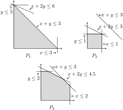
The inequality x + 3y ≤ (5a + 3)/2 is also redundant when a = 3 and a = 1, and the parameterized system R3 obtained by adding it to R2 entails R2. We can repeat the reasoning by adding infinitely many other inequalities, each time having a system that entails the previous one.

As suggested by the example, it is reasonable to limit the search space to generalizations whose inequalities over variables appear in some system Pi = Ai · x ≤ bi, for i = 1 . . .N, modulo normalization to unit length. Let ‖c‖ be the L2 norm of a vector c.

Definition 4.5 A vector c is generated from A1, . . . ,An if c = 0 or there is a row dT of some Ai, with i = 1 . . .N, such that c/‖c‖ = d/‖d‖.

A parameterized linear system P = C · x ≤ d +M · r is generated fromAi ·x ≤ bi, with i = 1 . . . N, if for every row cT · x ≤ d+mT · r in P, c is generated fromA1, . . . ,An.

We simply say that P is generated if the systems Ai · x ≤ bi are clear from the context. We are now in the position to define representativeness.

Definition 4.6 (Representativeness) A generalization is representative among those generated from Pi = Ai ·x ≤ bi, with i = 1 . . .N, if it is generated from P1, . . . , PN, and it entails any (parameter renamed apart) generalization generated from P1, . . . , PN.

Renaming apart parameters (i.e., substituting parameters with fresh ones) prevents clashing of parameters, and it allows for correctly applying Def. 3.2 of entailment.

4.3 The Base System

Inspired by the necessary condition of Lemma 4.3, we will be looking for a generalization starting from all distinct inequalities appearing in the input systems. Let us introduce first a key tool for characterizing parameter instances leading to a specific polyhedron.

Definition 4.7 (Maxima) Let A · x ≤ b be satisfiable linear system, and C·x ≤ d+M·r be a parameterized linear system

The maxima of C · x ≤ d +M · r w.r.t. A · x ≤ b is the vector k = (k1, . . . , kn) where ki, for i = 1 . . . n, is the solution of the linear program:

with n inequalities: cTi · x ≤ di +mTi · r, for i = 1 . . . n.

If any linear program is unbounded, the maxima is undefined.

Intuitively, ki is the value, if it exists, for which the hyperplane cTi · x = ki is incident to the polyhedron of A · x ≤ b. If Sol(A · x ≤ b) ⊆ Sol(C · x ≤ d +M · r, r0) for some r0, then it is necessarily the case that k ≤ d+M· r. Notice that the maxima does not depend on d nor on the parameters r, but only on the cone of the parameterized system, namely on C · x ≤ 0. Also, notice that the maxima can be computed in polynomial time, since it consists of solving n linear programs, each with polynomial complexity [Khachiyan, 1979].

Example 4.5 Consider the linear system 0 ≤ y, x + y ≤ 3, x ≤ 2. In the space of its solutions, the maximum value of -y is 0, of x+y is 3, and of x is 2. Therefore, the maxima of the parameterized system P consisting of -y ≤ a, x + y ≤ b, x ≤ c w.r.t. the linear system is (0, 3, 2). The instance of inequalities in P where the RHS is given by the maxima is: -y ≤ 0, x + y ≤ 3, x ≤ 2, which is precisely the original linear system. Differently from what this example may suggest, however, in general deciding whether a given linear system belongs to the class of a parameterized linear system is a NP-complete problem (see [Ruggieri, 2012]).

We are now ready to introduce the base system.

Definition 4.8 (Base system) Given N linear systems Pi = Ai · x ≤ bi such that Sol(Pi) ̸= ∅, with i = 1 . . .N, and called A = {c/‖c‖ | cT is a row in Ai for some i = 1, . . . ,N}, the base system is C · x ≤ r, 0 ≤ d +M · r where:

• C · x ≤ r is the set of inequalities cT · x ≤ r for every c ∈ A and with r fresh parameter;
• 0 ≤ d +M · r is the convex hull of k1, . . . , kN, where ki is the maxima of C · x ≤ r w.r.t. Ai · x ≤ bi, with i = 1 . . .N.

The base system is undefined if any of the ki's is undefined.

Intuitively, A is the set of LHS of inequalities in any of the input systems, normalized to unit length - e.g., x ≤ 0 and 2x ≤ 3 contribute to the same x ≤ r in C · x ≤ r. The maxima ki is the parameter instance for which C·x ≤ r leads to the polyhedron Sol(Ai · x ≤ bi) of the ith input system. Also, notice that the hypothesis that Sol(Ai · x ≤ bi) ̸= ∅ is required by the definition of maxima.

Example 4.6 Consider the following sample systems:

The base system P includes -y ≤ a, x + y ≤ b, x ≤ c plus (a linear system denoting) the convex hull of the three maxima (0, 3, 2), (0, 1, 1), and (0, 2, 2) over the space (a, b, c) of parameters, namely:

By construction [[P ]] includes the polyhedra of the sample systems. For instance, by fixing a = 0, b = 1, c = 1 we obtain 0 ≤ y, x + y ≤ 1, x ≤ 1, whose polyhedron is the same of the second system (the inequality x ≤ 1 is redundant).

By construction, the base system is generated from the input systems, and its class of polyhedra includes the ones of the input systems. Moreover, it entails any parameterized system satisfying such two properties.

Lemma 4.4 If the base system is defined, then it is a representative generalization.

Proof. Let P be C · x ≤ r, 0 ≤ d +M · r as in Def. 4.8. Also, let Pi be Ai · x ≤ bi for i = 1 . . .N.

Consider now representativeness. Let us show that P entails any Q that is a (renamed apart) generalization generated from P1, . . . , PN. Without any loss of generality, Q is of the form C′ · x ≤ t, 0 ≤ d′ +M′ · t, with t ∩ r = ∅, and C′ has unit rows. As a consequence, 0 ≤ d′ +M′ · t includes the convex hull of the maxima ti of C′ · x ≤ t w.r.t. Ai · x ≤ bi, namely ConvexHull(t1, . . . , tN). Let now r0 ∈ Sol(0 ≤ d +M · r). Since 0 ≤ d +M · r is a polytope, r0 can be written as a convex combination of its vertices, namely r0 = Σi=1...Nγiki, where Σi=1...Nγi = 1 and γi ≥ 0 for i = 1 . . . N. Let t0 = Σi=1...Nγiti. We claim that Sol(P, r0) ⊆ Sol(Q, t0). Let cT ·x ≤ t be the j th inequality of C′ · x ≤ t0. We show that Sol(P, r0) ⊆ Sol(cT · x ≤ t0) where t0 = Σi=1...Nγitij is the convex combination of the j th elements tij of t1, . . . , tN. Since Q is generated and C′ consists of unit rows, we have that any row cT of C′ is a row of C as well. This implies that max{cT · x0 | x0 ∈ Sol(P, ki)} = kij, where kij is the j th element of the maxima ki. Since Sol(P, ki) = Sol(Q, ti) ⊆ Sol(cT · x ≤ tij), this implies kij ≤ tij for i = 1 . . .N. This implies, Sol(P, r0) ⊆ Sol(cT · x ≤ Σi=1...Nγikij) ⊆ Sol(cT · x ≤ Σi=1...Nγitij) = Sol(cT · x ≤ t0). Summarizing, we conclude that P entails Q. □

P is clearly generated from P1, . . . , PN. Let us show it is a generalization. Let i = 1 . . .N, and ki be the maxima of C·x ≤ r w.r.t. Ai ·x ≤ bi. By definition of 0 ≤ d+M·r, we have that 0 ≤ d+M·ki holds, and then Sol(P, ki) = Sol(C· x ≤ ki). By definition of maxima, we have Sol(C · x ≤ ki) ⊇ Sol(Ai · x ≤ bi). Moreover, since C includes every row of A (possibly after normalization), we also have Sol(C· x ≤ ki) ⊆ Sol(Ai · x ≤ bi). Summarizing, Sol(P, ki) = Sol(Ai · x ≤ bi).

We are now in the position to show that the necessary condition of Lemma 4.3 for the existence of solutions to the learning problem is also sufficient.

Lemma 4.5 A generalization of P1, . . . , PN exists iff the base system of P1, . . . , PN is defined iff P1, . . . , PN have the same cone.

Proof. We split the proof into three claims.

(1) If a generalization exists then P1, . . . , PN have the same cone. This is Lemma 4.3.

(2) If P1, . . . , PN have the same cone then the base system is defined. We show the contrapositive. Assume there exists i = 1 . . .N and Sol(Ai · x ≤ bi) ̸= ∅ such that ki is undefined. This means that there exists j = 1 . . .N and Sol(Aj · x ≤ bj) ̸= ∅ such that for some row cT · x ≤ b in Aj · x ≤ bj it turns out that max{cT /‖c‖ · x | Ai · x ≤ bi} is unbounded. By the decomposition theorem of polyhedra [Schrijver, 1987], this implies that max{cT /‖c‖·x | Ai ·x ≤ 0} is unbounded. As a consequence, Sol(Aj · x ≤ 0) ̸= Sol(Ai · x ≤ 0) since max{cT /‖c‖ · x | Aj · x ≤ 0} is clearly bounded by 0.

(3) If the base system is defined then a generalization exists. This is precisely Lemma 4.4. □

Example 4.7 Consider the linear systems from Example 4.1. We have that C·x ≤ r in the base system is x ≤ a, y ≤ b. The maxima of C·x ≤ r w.r.t. the system x ≤ 0 is undefined since max{y |x ≤ 0} is unbounded. Hence there is no a, b such that x ≤ a, y ≤ b can lead to the polyhedron Sol(x ≤ 0).

4.4 TacklingMinimality: Parameter Elimination

The base system is a generalization and it is representative among those generated. Moreover, it is weakly minimal. This is an immediate consequence of the fact every parameter instance in its domain leads to a different polyhedron.

Lemma 4.6 Let P be the base system, and Sol(P, r0) ̸= ∅. For every, r0 ̸= r1 we have Sol(P, r0) ̸= Sol(P, r1).

Proof. The conclusion is immediate if Sol(P, r1) = ∅. Assume Sol(P, r1) ̸= ∅. Let r = ∑i=1...N λiki be any parameter instance in the convex hull of the maxima k1, . . . , kN (see Def. 4.8). We claim that r is the maxima of P w.r.t. Sol(P, r). This implies that if Sol(P, r0) = Sol(P, r1) then r0 = r1 because Sol(P, r0) ̸= ∅ and Sol(P, r1) ̸= ∅ imply that r0 and r1 are in the convex hull of k1, . . . , kN. Let us show our claim. Let cTj · x ≤ rj be the j th inequality in C· x ≤ r (see Def. 4.8). By definition of maxima, for i = 1 . . .N, there exists xi ∈ Sol(Pi) = Sol(P, ki) such that cTj · xij = kij. Called x′ = ∑i=1...N λixi, we have that:

Since cTj · x ≤ ∑i=1...N λikij is an inequality in P for parameters r = ∑i=1...N λiki, we conclude that ∑i=1...N λikij is the maximum of cTj ·x in Sol(P, r). Hence, ∑i=1...N λiki = r is the maxima of P in Sol(P, r). □

However, the base system is not necessarily strongly minimal nor minimal as per number of parameters. Example 4.6 suggests that the parameter a can be removed since a = 0 holds. A simple way of reducing parameters is Gaussian elimination restricted to parameter-only expressions.

Definition 4.9 The Gauss-elimination of a parameter r from a parameterized linear system P occurs if an equality r = d +mT · r is in P. The system obtained by replacing every occurrence of r in P by d +mT · r is denoted by G(P, r).

P is logically equivalent to G(P, r), r = d+mT ·r. Hence: [[P ]] = [[G(P, r), r = d +mT · r]] = [[G(P, r)]] ∪ {∅}. When P is the base system, ∅ ∈ [[P]] (since the domain of parameters is a polytope), and then [[P]] = [[G(P, r)]]. Moreover, since parameters are replaced by an expression of parameters only, G(P, r) is generated. Summarizing, the properties of being generated, representative, and weakly minimal are maintained for G(P, r), and this holds also for repeated applications of Gauss-elimination.

Example 4.8 Reconsider P from the Example 4.6. The parameter a can be eliminated, since a = 0 appears in P. G(P, a) is then 0 ≤ y, x + y ≤ b, x ≤ c, b ≤ 2c - 1, c ≤ 2, c ≤ b. G(P, a) is generated and [[P ]] = [[G(P, r)]].

More general variable elimination methods can also be applied, with the proviso that parameter elimination should result into a generated system. We ensure this by a syntactically restriction on the Fourier-Motzkin elimination procedure.

Definition 4.10 The restricted Fourier-Motzkin elimination of r from P occurs if all upper bounds on r in P involve parameters only, namely they can be written in of the form r ≤ d +mT · r, with r vector of parameters (not including r). The system obtained by Fourier-Motzkin-elimination of r from P is denoted by F(P, r).

In the Fourier-Motzkin elimination procedure (see [Schrijver, 1987]), every lower bound d1 +mT1 · r + cT · x ≤ r is replaced by inequalities d1+mT1 ·r+cT ·x ≤ d2+mT2 ·r for all upper bounds r ≤ d2 +mT2 · r. The syntactic restriction that variables do not appear in upper bounds maintains the property of being a generated system, yet being a sufficient condition only. It also implies:

and then F (P, r) entails P .

Example 4.9 Reconsider P ′ = G(P, a) from Example 4.8. Let us eliminate b. The only upper bound is b ≤ 2c - 1. Hence, F (P ′ , b) is 0 ≤ y, x + y ≤ 2c - 1, x ≤ c, 1 ≤ c, c ≤ 2. Let us instead eliminate c. There are two upper bounds c ≤ 2, c ≤ b. Hence, F(P ′ , c) is 0 ≤ y, x + y ≤ b, x ≤ 2, x ≤ b, 1 ≤ b, b ≤ 3. The inclusions [[P ′ ]] ⊇ [[F(P ′ , b)]] and [[P ′ ]] ⊇ [[F (P ′ , c)]] clearly hold by setting b = 2c-1 and c = min{2, b} in P ′ respectively.

Since the inclusion (1) can be strict, the property of being a generalization may be lost after restricted FourierMotzkin elimination. Thus, it has to be explicitly checked. Thanks to Lemma 4.6, F(P, r) is a generalization iff Sol(F(P, r), k′i ) = Sol(Pi) for i = 1 . . .N, where k′i is obtained by eliminating the r component from the vector of parameters ki such that Sol(P, ki) = Sol(Pi). Notice that such a condition can be checked in polynomial time, whilst the full membership procedure is NP-complete [Ruggieri, 2012]. In case F(P, r) is a generalization, it is representative (since (1) implies that F(P, r) entails P, which is representative) and weakly minimal (again by (1) and Lemma 4.6).

Example 4.10 Reconsider F(P ′ , b) from the Example 4.9. Recall that the maxima of the base system are (0, 3, 2),

(0, 1, 1) and (0, 2, 2). Their projection over the single parameter c in F(P ′ , b) is (2), (1), and (2). They lead to the following two instances of F(P ′ , b):

The polyhedron of the first sample system in Example 4.6 is not covered. Hence, F(P ′ , b) is not a generalization. As for F(P ′ , c), the projected maxima (3), (1), and (2) lead to:

Since x ≤ 1 and x ≤ 2 in the second and in the third systems are redundant, we obtain the polyhedra of the three sample systems of Example 4.6. Hence, F(P ′ , c) is a generalization, and then it is representative and weakly minimal.

Summarizing, a parameter elimination procedure consists of performing Gauss and restricted Fourier-Motzkin eliminations while possible. Gauss eliminations should be given priority since they remove inequalities, while not adding new ones. Restricted Fourier-Motzkin eliminations are performed only if they result in a generalization. The final system is a representative generalization and weakly minimal, yet not strongly minimal. However, strongly minimal generalizations do not necessarily define a unique class of polyhedra.

Example 4.11 Consider three linear systems:

The base system P includes x ≤ a, y ≤ b plus (a linear system denoting) the convex hull of the maxima (0, 0), (1, 2), and (2, 1) over the space (a, b) of parameters:

By eliminating the parameter b from P, we obtain Pb = F (P, b) consisting of x ≤ a, y ≤ 3 - a, y ≤ 2a, 0 ≤ a ≤ 2. Pb turns out to be a generalization: fix a = 0, a = 1, and a = 2 respectively for the three systems. Analogously, by eliminating a from P , we obtain Pa = F (P, a) consisting of x ≤ 2b, x ≤ 3 - b, y ≤ b, 0 ≤ b ≤ 2, which is a generalization as well. We observe that [[Pa]] ∩ [[Pb]] consists only of the polyhedra of the tree linear systems above. As a consequence, the strongly minimal generalization included in or equal to Pb and the one included in or equal to Pa necessarily define different classes of polyhedra.

5 Conclusions

We have introduced and investigated the problem of learning the definition of a class of polyhedra from sample polyhedral sets. Our approach consists of building a base system and then of eliminating parameters. Non-polynomial time steps include the computation of the convex hull of maxima and the use of the Fourier-Motzkin procedure in parameter elimination, which can be exponential in the worst case. An implementation of our approach has been developed in SWI-Prolog [Wielemaker et al., 2012], using a library on constraint logic programming (CLP) over the reals [Jaffar et al., 1992]. CLP offers powerful amalgamation features: linear systems can be represented using the language of constraints, thus exploiting language primitives for solving linear programming problems, entailments, simplifications, and so on. Source code can be downloaded from the home page of the author.