
Continuous Time Planning for Multiagent Teams with Temporal Constraints
Proceedings of the Twenty-Second International Joint Conference on Artificial Intelligence. Pages 465-470.
https://doi.org/10.5591/978-1-57735-516-8/IJCAI11-085
© 2011 International Joint Conferences on Artificial Intelligence
Abstract
Continuous state DEC-MDPs are critical for agent teams in domains involving resources such as time, but scaling them up is a significant challenge. To meet this challenge, we first introduce a novel continuous-time DEC-MDP model that exploits transition independence in domains with temporal constraints. Moreimportantly, we present a new locally optimal algorithm called SPAC. Compared to the best previous algorithm, SPAC finds solutions of comparable quality substantially faster; SPAC also scales to larger teams of agents.
- [Becker et al., 2003] R. Becker, S. Zilberstein, V. Lesser, and C. V. Goldman. Transition-independent decentralized Markov Decision Processes. In AAMAS, 2003.
- [Becker et al., 2004] R. Becker, S. Zilberstein, V. Lesser, and C. V. Goldman. Solving transition independent decen- tralized Markov Decision Processes. J. Artif. Int. Res., 22:423-455, 2004.
- [Benazera, 2007] E. Benazera. Solving decentralized contin- uous Markov decision problems with structured reward. In KI, 2007.
- [Bernstein et al., 2002] D. S. Bernstein, R. Givan, N. Immer- man, and S. Zilberstein. The complexity of decentralized control of Markov decision processes. Math. Oper. Res., 27:819-840, 2002.
- [Beynier and Mouaddib, 2005] A. Beynier and A. Mouad- dib. A polynomial algorithm for decentralized Markov decision processes with temporal constraints. In AAMAS, 2005.
- [Curtin and Bellingham, 2001] T. B. Curtin and J. G. Bellingham. Guest editorial -autonomous ocean-sampling networks. Oceanic Engineering, IEEE Journal of, 27, 2001.
- [Doshi et al., 2009] P. Doshi, Y. Zeng, and Q. Chen. Graph- ical models for interactive POMDPs: representations and solutions. JAAMAS, 2009.
- [Kumar and Zilberstein, 2010] A. Kumar and S. Zilberstein. Point-based backup for decentralized POMDPs: Com- plexity and new algorithms. In AAMAS, 2010.
- [Li and Littman, 2005] L. Li and M. Littman. Lazy approx- imation for solving continuous finite-horizon MDPs. In AAAI, 2005.
- [Marecki and Tambe, 2007] J. Marecki and M. Tambe. On opportunistic techniques for solving decentralized Markov decision processes with temporal constraints. In AAMAS, 2007.
- [Marecki and Tambe, 2009] J. Marecki and M. Tambe. Plan- ning with continuous resources for agent teams. In AA- MAS, 2009.
- [Marecki et al., 2007] J. Marecki, S. Koenig, and M. Tambe. A fast analytical algorithm for solving Markov decision processes with continuous resources. In IJCAI, 2007.
- [Nair et al., 2005] R. Nair, P. Varakantham, M. Tambe, and M. Yokoo. Networked distributed POMDPs: A synthesis of distributed constraint optimization and POMDPs. In AAAI, 2005.
- [Py et al., 2010] F. Py, K. Rajan, and C. McGann. A system- atic agent framework for situated autonomous systems. In AAMAS, Toronto, Canada, May 2010.
- [Spaan and Melo, 2008] M. T. J. Spaan and F. S. Melo. Interaction-driven Markov games for decentralized mul- tiagent planning under uncertainty. In AAMAS, 2008.
- [Wu et al., 2010] F. Wu, S. Zilberstein, and X. Chen. Point- based policy generation for decentralized POMDPs. In AAMAS, 2010.
References were extracted automatically from the PDF and may contain errors.
Full text extracted automatically from the PDF; figures, tables and equations may differ. The PDF is the version of record.
1 Introduction
Since the introduction of decentralized Markov Decision Processes (DEC-MDPs) to the field of multiagent systems over a decade ago, there has been significant progress in improving their efficiency [Becker et al., 2003; Kumar and Zilberstein, 2010; Wu et al., 2010]. Yet given the NEXP-complete complexity of DEC-MDPs [Bernstein et al., 2002] scaleup has been difficult. This challenge is further exacerbated in many real-world domains where we wish to apply DECMDPs: these involve continuous resources such as time or energy, and actions may involve uncertainty in their resource consumption (e.g. duration or energy consumption). And these domains often require that we deploy teams of agents, e.g. large numbers of autonomous underwater vehicles for scientific observations in the ocean [Curtin and Bellingham, 2001], unmanned aerial vehicles for surveillance or large autonomous mobile sensor webs deployed for disaster response.
The state-of-the-art in continuous time planning for DECMDPs often fails to meet this challenge. One of the latest algorithms, M-DPFP [Marecki and Tambe, 2009], is an attempt to find a global optimal for continuous time DEC-MDPs, where agents must coordinate over an unordered set of tasks. Unfortunately M-DPFP cannot scale-up beyond two agents and a handful of tasks. Other attempts in planning with continuous time for DEC-MDPs [Beynier and Mouaddib, 2005; Marecki and Tambe, 2007] have successfully solved problems with much larger number of tasks, but require that the task ordering be supplied ahead of time without a significant number of agents. There has been some success in scale-up in discrete state planning, in models such as ND-POMDPs [Nair et al., 2005] that exploit transition independence [Becker et al., 2003] and a network structure; for example ND-POMDPs have shown results for up to a dozen agents. While we build on some of the key ideas in ND-POMDPs, their discrete state approximation of continuous time domains can lead to significant degradation in solution quality (coarse-grained discretization) or very large inefficiencies (fine-grained discretization) [Marecki and Tambe, 2009].
This paper presents three key contributions. First, motivated by domains discussed in Section 2, we introduce a novel continuous-time DEC-MDP model (MCT-MDP) that exploits transition independence in domains with graphical agent dependencies and temporal constraints. Solving MCTMDP optimally remains difficult however, given that solving transition-independent DEC-MDPs with even discrete states is NP-Complete [Becker et al., 2004]. Our second contribution therefore presents a new iterative locally optimal algorithm called SPAC. The key idea in SPAC is a novel single-agent continuous-time MDP, called augmented CTMDP, such that solving it efficiently finds the best response of an agent to other agents' policies. SPAC's key novelties include: (i) fast convolution for creating an augmented CTMDP - creating this MDP itself is computationally challenging; (ii) enhancement of a previous single-agent continuoustime MDP algorithm [Li and Littman, 2005] to solve augmented CT-MDPs; (iii) exploiting graph structure of reward dependencies in MCT-MDP for scale-up. Finally, we empirically show that SPAC not only finds solutions substantially faster than M-DPFP with comparable quality, but also scales well to significantly larger team of agents.
2 Motivating Problem
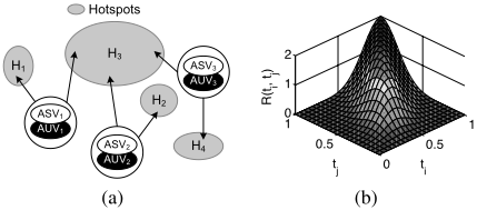
Our work is motivated by teams of robots, specifically Autonomous Underwater and Surface Vehicles (AUVs and ASVs) that coordinate to collect data from a coastal region [Py et al., 2010]. For example, Figure 1 shows a scenario where a team of three pairs of AUV/ASV is to collect sensor data and water samples in key biological hotspots. In Figure 1(a), H1, H2 and H4 are three small hotspots that require one pair of AUV/ASV each, while H3 is a large area that requires all three pairs to perform the sampling task simultaneously. While the ASVs take surface samples, their corresponding AUVs take underwater samples simultaneously. Actions such as traveling between hotspots, taking a sample, etc. may have uncertain durations. In this problem, one agent's action will not affect other agents' physical states.
Each single task has a reward associated with it; but the reward obtained may be based on the joint actions of multiple agents in the team. In particular, there are several types of temporal constraints within different sets of tasks. For example, we require the underwater samples to be taken simultaneously with the surface samples, which is modeled as a joint reward function. An example function is shown in Figure 1(b), where the ti and tj represent the remaining time when the two tasks are started and the R(ti, tj) represents the corresponding joint reward. We may also have precedence constraints that require one water sample to be taken before another, etc. Our goal in this and similar domains (with potentially much larger teams) is to compute an optimal plan that maximizes the team's total expected reward.
3 MCT-MDP
As our motivating domain illustrates, one agent's rewards may be dependent on other agent's state and actions, but its transitions are not. In DEC-MDP research, these types of transition-independent problems have been motivated earlier in many domains with discrete states [Becker et al., 2004; Nair et al., 2005]. To efficiently model time as part of an agent's local state, we formulate these types of planning problems as continuous-time transition-independent DEC-MDPs with soft temporal constraints. We first define a single-agent problem and then a decentralized one.
Definition 1. A single-agent continuous-time MDP (CTMDP) M is represented by a tuple 〈S, Δ, A, T, σ, R〉, where,
- S is a finite set of discrete states. s0 denotes the initial state.
- Δ = [0, t∗ ] is a one-dimensional continuous state representing the remaining time. The agent initially has t∗ remaining time. S × Δ defines the hybrid state space of the agent. We say the agent is at hybrid state 〈s, t〉, if its discrete state is s and remaining time is t.
- A is a finite set of actions. In addition, the agent can wait for an arbitrary amount of time. Wait action is denoted by φ (Wait is critical in multiagent settings, e.g. one agent may need to wait to perform its task as it may be dependent on another agent finishing its task).
- T : S×A×S ↦→R is the transition function of discrete states. T(s, a, s′ ) is the probability of entering s′ when action a is taken at state s.
- σ : Δ × S × A × S ↦→ R is the relative transition density function of the continuous states. σ(t|s, a, s′ ) is the probability density function (PDF) of the duration of taking action a at s and reaching s′ . We assume there is a minimum duration for all non-wait actions.
- R : Δ × S × A ↦→ R is the individual reward function. R(t|s, a) is the immediate reward obtained when the agent takes action a at hybrid state 〈s, t〉.
Definition 2. The policy π is a mapping from 〈s, t〉 to an action a. Denote such mapping by π(s, t) = a. We define the policy function απ(t|s, a):
Definition 3. An event e = 〈s, a〉, is a pair of a discrete state and a non-wait action. The set of all events E = S ×A. In this paper, we use e and 〈s, a〉 interchangeably.
Definition 4. Given policy π, fπ(t|e) is the PDF that event e happens with remaining time t.
The value of a policy π is the non-discounted expected reward of R: V (π) = ∑e∈E ∫ t∗ t=0 R(t|e)fπ(t|e)dt.
Definition 5. An n-agent transition-independent multiagent CT-MDP (MCT-MDP) is defined by 〈{Mi}, Ω, R〉.
- Mi = 〈Si, Δi = [0, t∗i ], Ai, Ti, σi, Ri〉 is the individual CT-MDP of agent i.
- Ω is a set of reward-dependent joint events. A joint event is denoted by ec, where c = {c1, . . . , c|c|} is a subgroup of agents and ec = {ec1 , . . . , ec|c| } is a joint event defined on c.
- For every ec ∈ Ω, R(tc1 , . . . , tc|c| |ec), defines the joint reward received if for every agent ci ∈ c, its event eci happens at tci .
Ω determines the graphical reward dependencies among agents, i.e. two agents are reward dependent if and only if there exists a joint event in Ω which comprises both agents' individual events. R captures the temporal constraint on dependent events by rewards. For example, R(t1, t2|e1, e2) is the reward function between e1 of agent 1 and e2 of agent 2. The global value of a joint policy π = {π1, . . . , πn} is the sum of non-discounted expected reward of both individual rewards Ri and joint rewards R. Thus,
Here πc = {πc1 , . . . , πc|c| } denotes the policies on subgroup c, where πci is the policy for agent ci. In this paper, we will represent R(t|e) by piecewise constant functions and R(tc1 , . . . , tc|c| |ec) by piecewise hyper-rectangular constant functions (values are constant in each hyperrectangles).
4 SPAC: Locally Optimal Algorithm
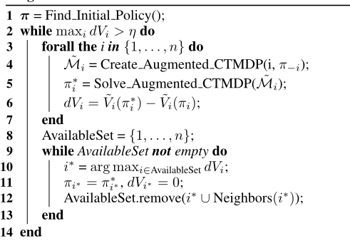
From an initial joint policy, SPAC (Scalable Planning for Agent teams under Continuous temporal constraints) obtains a locally optimal solution by iteratively finding the best response of one agent to its neighboring agents' policies. For finding a best response, a naive approach is to enumerate and evaluate all policies of the best-responding agent given fixed policies of its neighboring agents. However, this is infeasible in an MCT-MDP because first, there are infinite number of states given continuous remaining time; second, there are infinite number of decision choices since an agent can wait any amount of time. To address this difficulty, we present a novel augmented CT-MDP (defined below) to efficiently compute the best response of an agent. SPAC optimizes the joint policy as follows: (1) create the set of augmented CT-MDPs for each agent i with respect to other agents' policies π-i; (2) find new optimal policy π∗ i by solving the augmented CTMDP, and update the gain dVi = ˜ Vi(π∗ i ) - ˜ Vi(πi); (3) terminate if the maximum gain is smaller than a given threshold η, otherwise find a set of mutually reward independent agents with high overall gain greedily, update their policies from πi to π∗ i , and repeat the process from the first step. The pseudo code is shown in Algorithm 1. Next we will discuss the two sub-routines in Algorithm 1: (1) quickly create the augmented CT-MDP for an agent given its neighbors' policies (line 4); (2) solve it efficiently using piecewise constant approximations inspired by [Li and Littman, 2005] (line 5).
4.1 Fast Creation of Augmented CT-MDP
Definition 6. Given a MCT-MDP 〈{Mi}, Ω, R}〉 and a joint policy π, ˜Mi, the augmented CT-MDP of agent i, is the same as Mi except for the reward function, ˜Ri. ˜Ri(ti|ei) is the augmented reward function that sums up agent i's individual reward and all related joint rewards of an event ei,
The following Proposition shows that the optimal policy of the augmented CT-MDP for agent i given π-i is also the best response to π-i, i.e. it maximizes the global value function.
Proposition 4.1. Let π∗ i be the optimal policy of the augmented CT-MDP ˜Mi with respect to π-i. Then for agent i's any policy πi, we have, GV (π∗ i , π-i) ≥ GV (πi, π-i).
Proof. Let ˜ Vi(πi) be the expected value of ˜Mi with policy πi. After expanding and rearranging terms, we have,
Since for any πi, ˜ Vi(π∗ i ) ≥ ˜ Vi(πi), we have,
Proposition 4.1 shows augmented CT-MDPs are useful, however we still need fπ(t|e) to obtain ˜R via Equation (1). To obtain fπ(t|e) efficiently, we apply dynamic programming on decision steps:
Definition 7. If an agent takes a non-wait action, we say it takes one decision step. An agent is initially at decision step 0 and is at decision step k after taking k non-wait actions.
Considering the wait action as one decision step may result in an infinite number of decision steps since the agent can wait for an arbitrarily small amount of time. Hence in SPAC, we exclude the wait action from a decision step and treat it differently from any other actions (see below). Recall we assume all non-wait actions have a minimum duration. Thus, the maximum number of decision steps K can be bounded by the maximum number of non-wait actions that can be performed within the time limit t∗ .
Then we can define f (k) π (t|e) as the PDF of the remaining time when event e happens at decision step k. By definition we have, fπ(t|e) = ∑Kk=0 f (k) π (t|e). In addition, we define f (k) π (t|s) as the PDF of the remaining time when the agent enters s at decision step k. As the basis, we know at decision step 0, the agent is at s0 with remaining time t∗ , i.e. f (0) π (t|s) = 0 except f (0) π (t|s0 ) = δ(t - t∗ ), where δ(t) is the Dirac delta function. From decision step 0, f (k) π (t|e) and f (k) π (t|s) must be obtained using PDF propagation. To address the significant computational difficulties in this propagation due to the continuous functions and the wait action, our key ideas are to (a) approximate the continuous functions f and σ as piecewise constant (PWC) functions and (b) use Dirac delta functions to represent infinite probability density values due to the wait action. We first demonstrate these ideas using an example, followed by our formal definition.
Suppose there are two actions a1 and a2 available at s, both taking the agent to s′ with probability 1. f (k) π (t|s) is given by Figure 2(a), where the x-axis is the remaining time and yaxis is the probability density (In SPAC, f (k) π (t|s) is always a PWC function as shown later). The policy for s is to take a2 if the remaining time t ∈ (0, 0.25], wait if t ∈ (0.25, 0.75], and take a1 if t ∈ (0.75, 1]. We will show the procedures to obtain f (k) π (t|s, a1), f (k) π (t|s, a2), and f (k+1) π (t|s′ ). Getting f (k) π (t|s, a1) is straightforward as shown by the black line in Figure 2(c). Getting f (k) π (t|s, a2) is more difficult because of the wait action. If the agent enters s with t ∈ (0.25, 0.75], it will wait until the remaining time drops to 0.25 and then perform a2, implying that the non-wait action (a2) at 0.25 will inherit the probability mass related to the wait action. This exact point of remaining time (0.25) will have an infinite value in terms of a probability density function. To address this, we use Dirac delta functions in addition to the PWC function to properly represent all the infinite values, e.g. represented by a Dirac component at 0.25 in the corresponding PDF as shown in Figure 2(b). The PDF of performing a2 is the combination of a PWC function and a Dirac delta function as shown by the grey line in Figure 2(c). Knowing the PDF of the durations of both a1 and a2, we can calculate the PDF of entering s′ at step k + 1. The new PDF is a piecewise linear (PWL) function (dashed line in Figure 2(d)), and has to be approximated by a PWC function (solid line in Figure 2(d)) before the next iteration.
Formally, knowing the f functions for decision step k, we can apply the following equations to compute the f functions for decision step k + 1.
Equation (2) captures the two possibilities that the agent will take action a at 〈s, t〉: f (k) π (t|s)απ(t|s, a) is the PDF that the agent enters 〈s, t〉 and the policy of 〈s, t〉 is to take action a; g(k) π (t|s, a) represents the PDF that the agent enters 〈s, t′ 〉 with remaining time t′ > t and the policy indicates the agent should wait until the remaining time drops to t. To formally define g(k) π (t|s, a), we suppose given policy π and discrete state s, the agent should wait at L intervals {(t2l, t2l+1]} where t2l-1 < t2l < t2l+1 and l = 0, . . . , L1 (policy functions are always PWC when value functions are PWC, more details in the next subsection). Then g(k) π (t|s, a) can be written as the following,
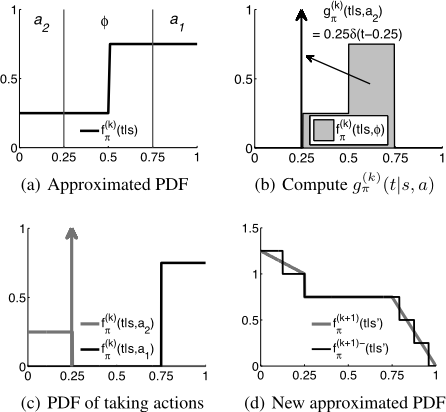
Here βa,l is the probability (not probability density) that the agent enters s at interval (t2l, t2l+1] and takes the non-wait action a at t2l. In PDF, this probability corresponds to a Dirac delta function at t2l with a magnitude equal to βa,l.
Since f (k) π (t|s) is a PWC function, f (k) π (t|s, a) obtained from Equation (2) is then the combination of a PWC function and a Dirac delta function. Equation (3) contains a convolution step between f(t) and the duration functions σ(t). Since duration functions are approximated by PWC functions, f (k+1) π (t|s′ ) computed by Equation (3) is a PWL function. At this point, we need to approximate f(t) by a PWC function f -(t) so that it can be used in the next iteration. Similar to [Li and Littman, 2005], the approximated PDF f -(t) is chosen such that the L∞ distance ‖f(t) - f -(t)‖∞ can be controlled by a given error bound ϵf > 0. In our experiments, we use fixed ϵf = 0.01.
At this point, fπ(t|e) can be obtained from summing up all f (k) π (t|e) over 0 ≤ k ≤K. Recall R(tc1 , . . . , tc|c| |ec) are piecewise hyper-rectangular constant functions, then the integral in Equation (1) returns a PWC function. Since Ri(ti|ei) are also PWC, then augmented reward functions ˜Ri are guaranteed to be PWC and can be directly used in solving the augmented CT-MDP as shown below.
4.2 Post-Creation: Solving Augmented CT-MDPs
To solve an augmented CT-MDP, we enhance Lazy Approximation [Li and Littman, 2005] to explicitly address the wait action. In particular, since the agent with remaining time t can wait until any t′ ≤ t with no cost, the optimal value for 〈s, t〉 is the maximum over the values of taking all possible actions a ∈ A at all possible continuous states t′ ≤ t.
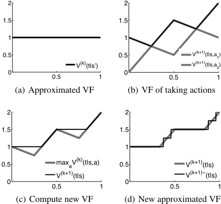
To first provide an intuitive explanation, we again demonstrate the overall process in Figure 3. Again suppose there are two actions a1 and a2 available at s, both taking the agent to s′ with probability 1. The value function of s′ at step k is as given by Figure 3(a). Figure 3(b) shows the value functions of taking a1 and a2 at s. The maximum of the two functions at t is the optimal value of taking an immediate action with t remaining time. Since the agent can let remaining time drop to any level t′ < t, the actual optimal value at t is the maximum of all values for all t′ < t as shown by the solid line in Figure 3(c). The new value function is however piecewise linear which then needs to be approximated by a PWC function before the next iteration. The solid line in Figure 3(d) shows the new value function after approximation. Formally, we have the following modified Bellman update,
where V (k) (t′ |s′ ) is the optimal value of s′ with remaining time t′ and k more decision steps. We approximate the optimal value functions V (t) by PWC functions. In Equation (5), ∫ t t′=0 V (t′ )σ(t-t′ )dt′ convolutes two PWC functions, V and σ, and returns a PWL function. Recall from the previous subsection, the augmented reward functions ˜R(t|s, a) are PWC functions. Therefore V (k+1) (t|s, a) obtained from Equation
(5) is a PWL function. Then maxa∈A V (k+1) (t|s, a) is also a PWL function, and therefore V (k+1) (t|s) obtained by Equation (4) is a PWL function. Similar to the last step in the previous subsection, we then approximate V (t) by a PWC function V -(t) so that the L∞ distance ‖V (t) - V -(t)‖∞ can be controlled by a given error bound ϵv > 0. ϵv is a key parameter our experiments test for efficiency tradeoffs.
5 Empirical Validation
We create a set of multiagent task allocation problems motivated by the real world domain described in Section 2. Each agent is assigned a disjoint set of tasks, corresponding to a disjoint set of actions ai. Each task i needs an uncertain amount of time to complete, whose distribution is denoted by σi. Completing task i before the deadline gains the team a reward of ri. We assume all the agents start execution at time 0 and share the same deadline of 1.0. For simplicity, we assume all tasks can be started from the beginning and must be completed before the deadline. An agent's discrete state can be represented by the set of tasks it has completed. We consider three types of binary temporal constraints (we omit the discrete state terms in R below for better readability).
(1) Precedence: The team gets a positive reward rij if task j is started after task i is completed. Let Pi(t) = ∫ t t′=0 σi(t′ )dt′ be the probability that task i can be completed in t amount of time. Then the constraint can be modeled by the corresponding joint component reward function,
(2) Simultaneity: The team receives a positive reward rij > 0 if the starting times of task i and task j are close enough.
(3) Exclusivity: The team receives a negative reward rij if the execution intervals of task i and task j overlap.
We first compare SPAC with M-DPFP, the only existing multiagent planner for unordered tasks and continuous resources. We test 2-agent problems with task values chosen uniformly randomly between 0 and 10. The task duration is fixed to a normal distribution N(0.3, 0.01). A total of two precedence constraints are added randomly. We vary the number of tasks assigned to each agent. For each setting, we create one problem instance and compare the runtime and final solution quality of SPAC and M-DPFP. For MDPFP we use approximation parameter κ = 0.25 and κ = 0.2 from [Marecki and Tambe, 2009]. For SPAC, we use ϵv = 1 and ϵv = 0.1 to allow tradeoffs between quality and runtime. Table 1 shows the total runtime of running SPAC 10 times with different random initial policies and the best solution among them. The first number of an entry is the runtime in seconds and the number in parentheses is the solution quality. NA indicates the algorithm fails to solve the problem within an hour. SPAC is seen to run substantially faster than M-DPFP and provides a comparable solution quality. For example, in the problem where each agent has 4 tasks, M-DPFP with κ = 0.2 finds a solution with quality of 27.7 in 247.6 seconds while SPAC with ϵv = 0.1 finds a better solution with quality of 34.7 in 0.6 seconds (412-fold speedup).
| #Tks | SPAC ϵv = 1 | SPAC ϵv = 0.1 | M-DPFP κ = 0.25 | M-DPFP κ = 0.2 |
| 3 | 0.1 (24.8) | 0.1 (26.0) | 0.4 (14.7) | 2.7 (16.4) |
| 4 | 0.4 (34.5) | 0.6 (34.7) | 21.7 (24.9) | 247.6 (27.7) |
| 5 | 0.4 (34.6) | 0.7 (34.9) | 63.2 (36.2) | NA |
| 6 | 0.6 (36.9) | 0.8 (38.2) | NA | NA |
Next, we conduct experiments to show SPAC's scalability. The task durations are chosen randomly from a set of pre-generated uniform distributions with mean in [0, 0.5] and variance of 0.01. Task values are chosen uniformly randomly between 0 and 10, and joint rewards are chosen uniformly randomly between 0 and 20 (-20 for penalties). The temporal constraints are randomly assigned between tasks.
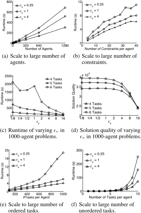
First we fix the number of tasks per agent to 5, the number of constraints per agent to 8, and vary the number of agents from 5 to 1280 with different error bounds ϵv = 0.25, 1, 4. For each setting we create 100 random problems and report the average runtime results in Figure 4(a). SPAC scales almost linearly with respect to the number of agents for every ϵv setting. Second, we fix the number of agents to 10, the number of tasks per agent to 5, and vary the number of constraints per agent. Again Figure 4(b) shows the average results over 100 random problems. As we can see, the runtime is roughly linear to the number of constraints per agent.
Next, we test on large scale problems where there are 1000 agents with 8 constraints per agent. We consider 4, 5, and 6 tasks per agent with varying ϵv from 0.125 to 16. Figure 4(c) and Figure 4(d) show the runtime and solution quality results of the average over 10 random problems respectively. The x-axes in both figures are in log-scale. These figures show that using smaller value of ϵv helps find better solutions at the cost of increasing runtime (however, the benefit of decreasing ϵv ≤ 0.5 is negligible). SPAC with ϵv = 0.5 is seen to solve a 1000 agent problem with 5 tasks per agent in 8 minutes - SPAC scales beyond capabilities of current algorithms.
Finally, we test the scalability with respect to the number of tasks per individual agent. To this end, we create 10-agent problems with 8 constraints per agent and varying number of tasks with task ordering either fixed or not fixed. If the task ordering is fixed, the number of discrete states of each agent is the number of tasks +1 and at each discrete state there is only one non-wait action. The problem with fixed task ordering is essentially to find an optimal starting time for the next task at every decision step. When the task ordering is not fixed, the problem is much more difficult - the number of discrete states is exponential to the number of tasks and the agent needs to choose one from the available tasks at each decision step. Figure 4(e) shows SPAC scales linearly with respect to the number of tasks per agent when the task ordering is fixed. It runs under 20 seconds for 1, 000 tasks, highlighting its scalability. However as shown in Figure 4(f), if the task ordering is not fixed, SPAC does not scale well - solving a problem with 10 unordered tasks per agent requires 250 seconds with ϵv = 0.25.
To test SPAC's solution quality - in the absence of an efficient global optimal solver - we run SPAC with ϵv = 0.25 for 5, 10, and 20 seconds and compare with best solution found in running SPAC with ϵv = 0.1 for 2 hours. As Table 2 shows, we can find good solutions with quality of at least 92% of the best by running SPAC for 5 seconds, and of at least 95% of the best by running SPAC for 20 seconds. Thus, SPAC can find reasonable solutions at a cheap computational cost.
| Id | 1 | 2 | 3 | 4 | 5 |
| 5s | 92.9% | 92.0% | 96.2% | 92.4% | 96.8% |
| 10s | 93.7% | 96.4% | 96.2% | 97.9% | 98.4% |
| 20s | 95.6% | 96.4% | 96.2% | 97.9% | 99.2% |
6 Conclusion
This paper presents three key contributions. First, it introduces a novel continuous-time model (MCT-MDP) for multiagent planning that exploits transition independence in domains with graphical reward dependencies and temporal constraints. Second, it presents SPAC, a new locally optimal algorithm, based on the following key ideas: (1) defining an augmented CT-MDP such that solving it provably provides a best response to neighboring agents's policies; (2) fast convolution to efficiently generate augmented CT-MDPs; (3) a new algorithm to solve these augmented MDPs; (4) exploiting graph structure of reward dependencies for scalability. Third, we show empirically that SPAC outperforms the nearest competitor (M-DPFP) and scales up the number of agents significantly beyond any previous continuous state DEC-MDP algorithm.
As for related work, there have been many algorithms proposed for solving discrete state DEC-MDPs and DECPOMDPs such as [Becker et al., 2003; Kumar and Zilberstein, 2010]. However, these techniques usually cannot be easily applied to continuous state problems. On the other hand, there are algorithms for solving hybrid state MDPs such as [Li and Littman, 2005; Marecki et al., 2007], which however, only solve for single-agent problems. Algorithms such as [Benazera, 2007; Beynier and Mouaddib, 2005; Marecki and Tambe, 2007; 2009] have been successful in solving multi-agent planning problems with continuous states. Unfortunately, [Beynier and Mouaddib, 2005; Marecki and Tambe, 2007] consider only a restricted problem where a fixed ordering of agent actions is given. Our experimental results show that when task ordering is supplied ahead of time, SPAC's scale-up is comparable or superior to that of these algorithms; however, SPAC can also handle unordered tasks which these algorithms cannot handle. The exponential complexity of M-DPFP [Marecki and Tambe, 2009] limits its applicability to only small problems. The goal-oriented joint reward structure in [Benazera, 2007] cannot represent the temporal constraints in our problems. Furthermore, none have been shown to scale to large numbers of agents. The MCT-MDP model introduced in this paper is a continuous state generalization of the TI-DEC-MDP model introduced by Becker et al. [Becker et al., 2003]. Unfortunately the coverage set algorithm (CSA) introduced in [Becker et al., 2003] cannot directly solve the continuous state model given that there are an infinite number of policies for an individual agent. We notice there exist efficient discrete state graphical models of agent interactions including [Doshi et al., 2009] and [Spaan andMelo, 2008]. Integrating such graphical representations to our model can be an interesting future research topic.
7 Acknowledgements
This research was supported by a subcontract from Perceptronics Inc. We thank Kanna Rajan for detailed comments and discussions.
@inproceedings{ijcai2011p85,
  title     = {Continuous Time Planning for Multiagent Teams with Temporal Constraints},
  author    = {Yin, Zhengyu and Tambe, Milind},
  booktitle = {Proceedings of the Twenty-Second International Joint Conference on
               Artificial Intelligence, {IJCAI-11}},
  publisher = {AAAI Press/International Joint Conferences on Artificial Intelligence},
  editor    = {Toby Walsh},
  pages     = {465--470},
  year      = {2011},
  month     = {7},
  doi       = {10.5591/978-1-57735-516-8/IJCAI11-085},
  url       = {https://doi.org/10.5591/978-1-57735-516-8/IJCAI11-085},
}
TY - CPAPER TI - Continuous Time Planning for Multiagent Teams with Temporal Constraints AU - Yin, Zhengyu AU - Tambe, Milind T2 - Proceedings of the Twenty-Second International Joint Conference on Artificial Intelligence, IJCAI-11 PB - AAAI Press/International Joint Conferences on Artificial Intelligence PY - 2011 SP - 465 EP - 470 DO - 10.5591/978-1-57735-516-8/IJCAI11-085 UR - https://doi.org/10.5591/978-1-57735-516-8/IJCAI11-085 ER -Copied
Machine-readable versions of this paper, for tools and AI agents:





