Finding (α, ϑ)-Solutions via Sampled SCSPs

1 Introduction

In a stochastic constraint satisfaction problem (SCSP) one typically requires a number of constraints, involving decision and random variables, to be satisfied at a prescribed probability. These constraints, which we call chance-constraints, take the form Pr{〈constraint〉} ≥ β and they enforce the probability 〈constraint〉 is satisfied by a given assignment to be greater or equal to a given threshold β. Typically, these constraints do not admit a closed form solution and are complex enough to rule out any chance of obtaining an exact solution via standard scenario-based approaches - for instance because they constrain random variables defined over a continuous support. We argue that a decision maker, instead of looking for an exact solution, may then aim to "estimate" for the chance-constraints in the model, the satisfaction probability guaranteed by a given assignment. In other words, having introduced a confidence level α and a tolerance threshold ϑ, the decision maker may look for a solution that, with confidence level α, guarantees a satisfaction probability that is no lower than β-ϑ. By choosing different values for α and ϑ the set of solutions may vary. For this reason, we will introduce a new notion of solution that is parameterized by these two parameters and that we call an (α, ϑ)-solution. Intuitively, as α tends to 1 and ϑ tends to 0 the set of (α, ϑ)-solutions will converge to the actual set of solutions to the original SCSP, which we therefore rename (1, 0)-solutions. In this work, we formally introduce the concept of (α, ϑ)-solution and we apply it to SCSPs that include continuous random variables - i.e. an infinite number of scenarios - and that cannot be solved by exact approaches in the stochastic constraint programming literature.

2 Formal Background

An m-stage SCSP [Walsh, 2002; Tarim et al., 2006; Hnich et al., 2009] is defined as a 7-tuple 〈V, S, D, P, C, β, L〉, where V is a set of decision variables and S is a set of random variables, D is a function mapping each element of V (respectively, S) to a domain (respectively, support) of potential values. In classical SCSPs both decision variable domains and random variable supports are assumed to be finite. P is a function mapping each element of S to a probability distribution for its associated support. C is a set of chance-constraints over a non-empty subset of decision variables and a subset of random variables. β is a function mapping each chanceconstraint h ∈ C to βh which is a threshold value in the interval (0, 1]. L = [〈V1, S1〉, . . . , 〈Vi, Si〉, . . . , 〈Vm, Sm〉] is a list of decision stages such that each Vi ⊆ V , each Si ⊆ S, the Vi form a partition of V , and the Si form a partition of S.

To solve an m-stage SCSP an assignment to the variables in V1 must be found such that, given random values for S1, assignments can be found for V2 such that, given random values for S2, . . ., assignments can be found for Vm so that, given random values for Sm, the hard constraints are satisfied and the chance constraints are satisfied in the specified fraction of all possible scenarios. Under the assumption that random variable supports are finite, the solution of an m-stage SCSP is, in general, represented by means of a policy tree [Tarim et al., 2006]. The arcs in such a policy tree represent values observed for random variables whereas nodes at each level represent the decisions associated with the different stages. We call the policy tree of an m-stage SCSP that is a solution a satisfying policy tree.

In order to simplify the presentation, we assume without loss of generality, that each Vi = {xi} and each Si = {si} are singleton sets. All the results can be easily extended in order to consider |Vi| > 1 and |Si| > 1 (see [Hnich et al., 2009]). Let S = {s1, s2, . . . , sm} be the set of all random variables and V = {x1, x2, . . . , xm} be the set of all decision variables. Let p be a path from the root node of the policy tree to a leaf. Let Ψ denote the set of all distinct paths of a policy tree. For each p ∈ Ψ, we denote by arcs(p) the sequence of all the arcs in p whereas nodes(p) denotes the sequence of all nodes in p. We denote by Ω = {arcs(p)|p ∈ Ψ} the set of all scenarios of the policy tree. The probability of ω ∈ Ω is given by Pr{ω} = ∏mi=1 Pr{si = ¯ si}, where Pr{si = ¯ si} is the probability that random variable si takes value ¯ si .

Now consider a chance-constraint h ∈ C with a specified threshold level βh. Consider a policy tree T for the SCSP and a path p ∈ T . Let h↓p be the deterministic constraint obtained by substituting the random variables in h with the corresponding values (¯ si) assigned to these random variables in arcs(p). Let ¯h↓p be the resulting tuple obtained by substituting the decision variables in h↓p by the values (¯xi) assigned to the corresponding decision variables in nodes(p). We say that h is satisfied wrt to a given policy tree T iff

Definition 1 Given an m-stage SCSP P and a policy tree T , T is a satisfying policy tree to P iff every chance-constraint of P is satisfied wrt T .

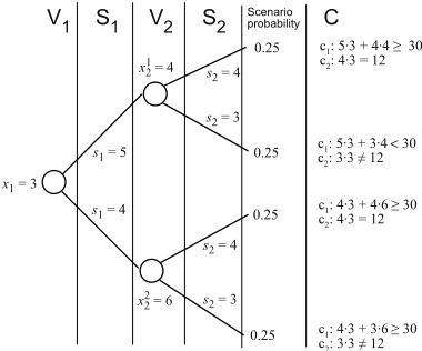
Example 1 Let us consider a two-stage SCSP in which V1 = {x1} and S1 = {s1}, V2 = {x2} and S2 = {s2}. Random variable s1 may take two possible values, 5 and 4, each with probability 0.5; random variable s2 may also take two possible values, 3 and 4, each with probability 0.5. The domain of x1 is {1, . . . , 4}, the domain of x2 is {3, . . . , 6}. There are two chance-constraints in C, c1 : Pr{s1x1 + s2x2 ≥ 30} ≥ 0.75 and c2 : Pr{s2x1 = 12} ≥ 0.5. In this case, the decision variable x1 must be set to a unique value before random variables are observed, while decision variable x2 takes a value that depends on the observed value of the random variable s1. A possible solution to this SCSP is the satisfying policy tree shown in Fig. 1 in which x1 = 3, x12 = 4 and x22 = 6, where x12 is the value assigned to decision variable x2, if random variable s1 takes value 5, and x22 is the value assigned to decision variable x2, if random variable s1 takes value 4. As the example shows, a solution to a SCSP is not simply an assignment of the decision variables in V to values, but it is instead a satisfying policy tree.

3 Existing Approaches for Modeling and Solving SCSPs

In [Tarim et al., 2006], the authors discuss an equivalent scenario-based reformulation for SCSPs. This reformulation makes it possible to compile SCSPs down into conventional (non-stochastic) CSPs. The scenario-based reformulation approach allows us to exploit the full power of existing constraint solvers. However, as pointed out in [Hnich et al., 2009], it has a number of serious drawbacks that might prevent it from being applied in practice: weakened constraint propagation and significant space requirements. In [Hnich et al., 2009] an alternative approach based on global chanceconstraints was proposed. Global chance-constraints were introduced first in [Rossi et al., 2008] and bring together the reasoning power of global constraints from constraint programming and the expressive power of chance-constraints from stochastic programming. The approach in [Hnich et al., 2009] is able to reuse existing propagators available for the respective deterministic global constraint obtained when all the random variables are replaced by constant parameters.

Unfortunately, both the above approaches operate under the assumption that the number of scenarios must be finite, otherwise a policy tree would comprise an infinite number of paths. This, in turn, means that complete approaches such as the one in [Tarim et al., 2006] and in [Hnich et al., 2009] can only deal with random variables having finite supports. Furthermore, these approaches do not scale well, since even problems having a limited number of random variables with large support immediately produce policy trees whose size makes impractical the use of a complete method.

In practice, it is often the case that random variables either range over continuous supports or have a very large number of possible values in their domain. In [Tarim et al., 2006], the authors therefore proposed to employ a number of sampling strategies in order to reduce a-priori the support of random variables and therefore produce SCSPs that are manageable. Nevertheless, their approach is purely heuristic and does not provide any likelihood guarantee on the quality of the assignments produced. The same holds for other heuristic approaches in the literature, such as the one in [Prestwich et al., 2009], in which a neural network is employed in order to encode a policy function that takes the best possible decision with respect to the past history of decisions taken and values observed for the random variables.

In the rest of this work we will discuss an effective way of dealing with single-stage SCSPs comprising random variables with continuous or very large support. This approach exploits sampling in order to keep under control the amount of scenarios that must be analyzed in order to find a solution. Intuitively, our approach "estimates" if a given assignment is consistent or not with respect to a given set of chanceconstraints. As in statistical estimation, the quality of this estimate is determined by confidence interval analysis. In contrast to [Tarim et al., 2006], we provide likelihood guarantees for the solutions found. In fact, we explicitly indicate a confidence probability that bounds the actual probability of making a wrong estimation. Before discussing our approach, we now introduce the concept of "sampled SCSP".

4 Sampled SCSPs

Consider a SCSP P over a set S of random variables. Assume that random variables are defined on continuous or large discrete supports. Solving the original SCSP clearly poses a hard combinatorial challenge, in fact the policy tree comprises a number of scenarios that is exponential in the size of random variable domains. Furthermore, if the random variable support is continuous, the policy tree comprises an infinite number of scenarios. In this section we discuss how to sample a more compact SCSP, which comprises at most N scenarios, out of the original problem. We shall call this new problem ̂ PN or "sampled SCSP" over N scenarios. Intuitively, a sampled SCSP is a reduced version of the original problem, the solution of which is a policy tree that comprises a bounded number of paths sampled out of the original policy tree. In the following sections we will discuss under which conditions the solution to ̂ PN is, with a prescribed confidence probability, likely to be also a solution to the original SCSP P.

We now discuss how to employ Simple Random Sampling to obtain a sampled SCSP out of the original problem. Of course, more advanced stratified sampling techniques may be used in order to reduce variance and improve the effectiveness of the approach. Nevertheless, we leave this discussion as future work.

Consider a complete realization, ¯ s1, . . . , ¯ sm, for the random variables in S obtained by sampling a value from the support D(si) of each of the random variables si ∈ S according to its probability distribution P(si). From the definition of policy tree it is clear that there always exists a path associated with this realization. In other words, this realization corresponds to one of the scenarios comprised in the policy tree. Consider a policy tree T for P and N complete sets of random variable realizations generated independently: {¯ s11 , . . . , ¯ s1m}, {¯ s21, . . . , ¯ s2m}, . . . , {¯ sN1 , . . . , ¯ sNm}, where ¯ sij is the realized value for random variable j observed in the ith set of realizations. We remove from T every path which corresponds to an arc labeling not observed in the former N complete realizations. Let ̂ T be the reduced policy tree. ̂Ψ denotes the reduced set of distinct paths in ̂ T . The probability of each of the remaining path p ∈ ̂Ψ, i.e. Pr{arcs(p)}, is simply set equal to the frequency of occurrence of such a path in the above N realizations. Of course, ̂ T represents a policy tree for a different SCSP than the one we started with. We call this new problem the sampled SCSP ̂ PN. Now consider a chance-constraint h ∈ C with a specified threshold level βh, a policy tree ̂ T for the sampled SCSP ̂ PN and a path p ∈ T . We say that h is satisfied wrt to a given policy tree ̂ T iff

Example 2 Let us consider the two-stage SCSPP discussed in Example 1. We set N = 3 and we derive a sampled SCSP ̂ PN. By using simple random sampling we draw the following three complete realizations for random variables in P: {¯ s11 = 5, ¯ s12 = 4}, {¯ s21 = 4, ¯ s22 = 4}, {¯ s31 = 5, ¯ s32 = 4}. A possible solution to the sampled SCSP ̂ PN is the satisfying policy tree shown in Fig. 2, in which x1 = 3, x12 = 4 and x22 = 6, where x12 is the value assigned to decision variable x2, if random variable s1 takes value 5, and x22 is the value assigned to decision variable x2, if random variable s1 takes value 4. The above policy tree has two paths sampled out of the original tree: p1 has an associated probability of 2/3, since we observed two occurrences of the scenario associated with this path over the 3 complete realizations sampled for the random variables; p2 has an associated probability of 1/3, since we observed a single occurrence of the scenario associated with this path over the 3 complete realizations sampled for the random variables. Paths that were not observed in the sampled realizations have an associated probability equal to 0 and are not considered.

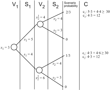
It should be noted that every policy tree ̂ T for a sampled SCSP ̂ P can be employed as a (partial) policy tree for the original SCSP P. Nevertheless, by sampling we lose completeness. If at stage i in P we observe, for a given random variable, a realized value that is not comprised in ̂ T , it will be of course impossible to determine the correct decisions for subsequent stages. This means that all paths in the corresponding subtree will never be satisfied. In multi-stage SCSPs, and especially in those including random variables with continuous support, this is a critical issue that prevents the direct use of the approach discussed in this work. It is therefore essential to adopt a "rolling horizon" approach [Sethi and Sorger, 1991] in order to reduce the multi-stage SCSPs to a sequence of single-stage SCSPs. For space reasons, we leave this discussion as future work. In general, however, it is possible that the remaining paths form a (partial) policy tree that is a satisfying policy tree for P. In Example 2, incidentally, the satisfying policy tree for the sampled SCSP is also a satisfying policy tree for the original SCSP. It is relatively intuitive to see that if we repeatedly produce new sampled SCSPs with N = 3, with a certain probability a satisfying policy tree for the sampled SCSP will also be a satisfying policy tree for the original SCSP. The rest of this work is mainly concerned with the estimation of this probability for single-stage SCSPs. We next introduce the relevant background in confidence interval analysis, the key tool we employ to perform this estimation.

5 Confidence Interval Analysis

Confidence interval analysis is a well established technique in statistics. Informally, confidence intervals are a useful tool for computing, from a given set of experimental results, a range of values that, with a certain confidence level (or confidence probability), will cover the actual value of a parameter that is being estimated.

Consider a discrete random variable that follows a Bernoulli distribution. Accordingly, such a variable may produce only two outcomes, i.e. "yes" and "no", with probability q and 1 - q, respectively.

Let us assume that the value q - the "yes" probability - is unknown. Obviously, if we observe the outcome of a Bernoulli trial once, the data collected will not reveal much about the value of q. Nevertheless, in practice, we may be interested in "estimating" q, by repeatedly observing the behavior of the random variable in a sequence of Bernoulli trials. This problem is well-known in statistics and both exact and approximate techniques are available for performing this estimation [Clopper and Pearson, 1934; Agresti and Coull, 1998]. The estimation produced by the methods available in the literature typically does not come as a point estimate, rather it consists of an interval of values computed from a set of representative samples for the quantity being estimated. This interval is known as "confidence interval" and consists of a range of values that, with a certain confidence probability α, covers the actual value of the parameter that is being estimated.

A method that is commonly classified as the "exact confidence intervals" for the Binomial distribution has been introduced by Clopper and Pearson in [Clopper and Pearson, 1934]. This method uses the Binomial cumulative distribution function (CDF) in order to build the interval from the data observed. The Clopper-Pearson interval can be written as (plb, pub), where

X is the number of successes (or "yes" events) observed in the sample, Bin(N; q) is a binomial random variable with N trials and probability of success q and α is the confidence probability. Note that we assume plb = 0 when X = 0 and that pub = N when X = N.

Because of the close relationship between Binomial distribution and the Beta distribution, the Clopper-Pearson interval is sometimes presented in an alternative format that uses percentiles from the beta distribution [Evans et al., 2000]:

where BetaInv denotes the inverse Beta distribution. This form can be efficiently evaluated by existing algorithms.

An interesting property of confidence intervals related to the estimation of the "success" probability associated with a Bernoulli trial consists in the fact that, given a confidence probability, it is possible to derive mathematically, by performing a worst case analysis, the minimum number of samples that should be observed in order to produce a confidence interval of a given size.

Therefore, for a given confidence probability α, it is possible to determine the minimum number of samples that should be considered in order to achieve a margin of error of ±ϑ in the estimation of the "success" probability of a Bernoulli trial. This computation plays a central role in our novel approach. In fact, intuitively estimating the satisfaction probability of a chance-constraint is equivalent to estimating the "success" probability of the associated Bernoulli trial.

6 Properties of Sampled SCSP Solutions

We will now characterize the probability that the solution of a sampled SCSPs ̂ PN over N scenarios, which may be computed by using any of the existing approaches discussed in Section 3, is a solution to the original single-stage SCSP P.

We will firstly discuss what the minimum value for N is in order to achieve a predefined probability α that a given policy tree T that satisfies a chance-constraint h in the sampled SCSPs ̂ PN also satisfies the same chance-constraint in the original SCSP P. Since a policy tree T in ̂ PN by definition only comprises a subset ̂Ψ of all the paths that constitute a policy tree for the original SCSP P, this policy tree, in order to satisfy h in the original SCSP P, must clearly provide a sufficient satisfaction probability regardless of the scenarios that have been ignored by the sampling process.

Consider a confidence probability α and a margin of error of ±ϑ; The number of scenarios N for the sampled SCSP depends on ϑ, α and also β, which we recall is the satisfaction probability we aim for our chance-constraint h.

Definition 2 N is computed as the minimum value for which

where (pβlb , pβub ), is the Clopper-Pearson confidence interval for a confidence probability ̂α, where ̂α = 2α - 1, 1 and round(βN) "successes" in N trials; round() approximates the value to the nearest integer. 2

Definition 3 Any policy tree T , which can be proved to satisfy h in P with probability α, satisfies h in P with probability α if it satisfies h in ̂ PN. Conversely, any policy tree T , which can be proved to not satisfy h in P with probability α, does not satisfy h in P with probability α, if it does not satisfy h in ̂ PN .

Proposition 1 A policy tree T can be proved to satisfy h in P with probability α if the actual satisfaction probability δ > β provided by T wrt h is such that δ ≥ pβub . Conversely, if the actual satisfaction probability δ < β provided by T wrt h is such that δ ≤ pβlb T can be proved to not satisfy h in P with probability α.

1 This transformation is required because Clopper-Pearson interval is a symmetric two-sided confidence interval, while when we determine if a policy tree satisfies or not a given chance-constraint we do this on the basis of a single-sided interval.

2 This is justified by the fact that the Clopper-Pearson interval is, in fact, a step function - see [Clopper and Pearson, 1934], p. 405 - since the Binomial is a discrete probability distribution.

Proof: Let δ ≥ pβub . By definition,

pβub = max{q| Pr{Bin(N; q) ≤ round(βN)} ≥ (1 - ̂α)/2. Therefore, it is clear that Pr{Bin(N; δ) ≤ round(βN)} < 1 - α. This means that

where we recall that ̂Ψ is the set of paths in the sampled SCSP ̂ PN. This implies

Therefore, by using the test

a policy tree T can be proved to satisfy h in P with probability α. Conversely, let δ ≤ pβlb . By definition,

Therefore, it is clear that

This means that

which implies

Therefore, by using the test

a policy tree T can be proved to not satisfy h in P with probability α. □

Proposition 2 Any policy tree T which provides a satisfaction probability δ ≥ β +ϑ wrt h in P can be proved to satisfy h in P with probability α. Any policy tree T which provides a satisfaction probability δ ≤ β -ϑ wrt h in P can be proved to not satisfy h in P with probability α.

Proof: this directly follows from Definition 2 and Proposition 1. □

Proposition 3 Any policy tree T which can not be proved to satisfy or to not satisfy h in P with probability α, can be either proved to satisfy h in P with probability γ, where γ is a probability ranging in (0.5, α(, if it satisfies h in ̂ PN, or to not satisfy h in P with probability γ, where γ is a probability ranging in (0.5, α(, if it does not satisfies h in ̂ PN .

Proof: Consider the two limiting cases. (i) The actual satisfaction probability δ provided by T wrt h in P is exactly equal to β. Since the sample mean, used to estimate the satisfaction probability out of the N samples considered, is an unbiased estimator of δ, it will overestimate β with probability 0.5 and, similarly, it will underestimate β with probability 0.5; this sets the lower bound for γ. (ii) The actual satisfaction probability δ provided by T wrt h in P is exactly equal to β + ϑ. From the proof of Proposition 1 it immediately follows that, in this case, γ = α, and also that, if δ < β +ϑ then γ < α; this sets the upper bound for γ.□

Definition 4 An (α, ϑ)-solution to a SCSP P is a policy tree ̂ T that at least with probability α provides for every chanceconstraint hi in P with satisfaction threshold βi a satisfaction probability greater or equal to βi - ϑ.

It is apparent that ϑ may be interpreted as a parameter that the user can set in order to define a "region of indifference", i.e. β ± ϑ, for the satisfaction probability. In such a region, we assume that assignments can be safely misclassified with probability greater than α and that satisfaction probabilities remain in an acceptable range.

6.1 Example

Consider the single-stage SCSP P = 〈V, S,D, P,C, β, L〉, where V = {X1,X2}, S = {r1, r2}, D(X1) = D(X2) = {0, 1}, D(r1) = (0, 100), P(r1) = Uniform(0, 100), D(r2) = (0, 300), P(r2) = Uniform(0, 300), C = {c : C1 ≥ X1r1 +X2r2}, βc = 0.5, and L = [〈V, S〉]. C1 = 185 is a constant. This problem comprises random variables defined on a continuous support and it cannot be solved by existing complete approaches to SCSPs. If we set α = 0.95 and ϑ = 0.05, from Definition 2 we compute the number of samples N = 250 required to guarantee that any solution to the sampled SCSP ̂ P over N samples is an (α, ϑ)-solution for P.

Furthermore, the simple structure of the constraint c considered in P allows us to perform some further analysis. Consider the assignment X1 = 1 and X2 = 1. A simple reasoning on the convolution of two independently non-identically distributed uniform random variables (see [Sadooghi-Alvandi et al., 2009]) immediately suggests that this assignment is indeed inconsistent. r1 and r2 are two independently non-

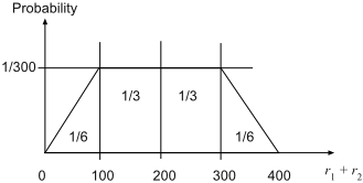
identically distributed uniform random variables. The distribution that results from their convolution is shown in Fig. 3. This distribution is shaped like a trapezoid. Clearly, since the area for the whole figure must be equal to 1, the area of each of the two rectangle triangles at the side of the trapezoid must be equal to 1/6. Consequently, the area of the internal rectangle must be equal to 2/3. It is easy to see that the cumulative distribution function for value 200 returns a probability of 0.5. Then, since 1/3*(15/100)=0.05, the 0.45 quantile of the inverse cumulative distribution function which results from convoluting r1 and r2 is exactly equal to C1 = 185. Therefore, since the satisfaction probability provided by the assignment X1 = 1 and X2 = 1 is equal to βc - ϑ = 0.45, this assignment will be correctly classified as inconsistent with probability α, when the sample size is set to N = 250.

6.2 Multiple Chance-constraints

Let h1, . . . , hk be k chance-constraints in a SCSP P. Let ̂ P be a sampled SCSP over N samples, where N is the number of samples required to guarantee a confidence level α and an error tolerance threshold ϑ for each constraint hi considered independently, according to Definition 2.

Proposition 4 Let ̂ T be a policy tree that is a solution to ̂ P. Then ̂ T is an (α, ϑ)-solution for P.

Proof: Consider a chance-constraint hi. Let βi be the respective satisfaction threshold. By definition, the probability that a solution ̂ T to ̂ P provides a service level less or equal to βi - ϑ for hi in P is less or equal to 1 - α. Therefore ̂ T is an (α, ϑ)-solution. Now consider a pair of chance-constraints 〈hi, hj〉 with satisfaction thresholds βi, βj, respectively. The probability that a solution ̂ T to ̂ P provides a service level less or equal to βi - ϑ for hi and to βj - ϑ for hj in P is less or equal to (1-α)2 , in fact we must misclassify both the constraints in order to accept such a solution. Even a single constraint correctly classified will make ̂ T inconsistent w.r.t. ̂ P. This reasoning can be easily generalized to k chanceconstraints, for which the probability becomes (1-α)k . Noting that (1 - α)k < . . . < (1 - α)2 < (1 - α) and that 1 - (1 - α)k ≥ α the probability that a solution is misclassified in a model comprising a single constraint, i.e. (1 - α), represents an upper bound for the probability that a solution ̂ T to ̂ P does not provide a satisfaction probability within the required tolerance threshold for one or more constraints in a generic model P. By rephrasing, the probability that a solution ̂ T provides a satisfaction probability greater or equal to βi -ϑ for each constraint hi is greater or equal to α. Therefore, by Definition 4, ̂ T is an (α, ϑ)-solution for P. □

Our approach is quite conservative and it will often attain a confidence probability greater than α for a generic model with k chance-constraints, since several assignments will typically violate more chance-constraints. However, when the number of chance-constraints increases, also the probability of misclassifying solutions increases, and we may need a higher confidence α to find one.

7 Conclusions

We proposed a framework for exploiting sampling in order to solve single-stage SCSPs that include random variables over a continuous or very large discrete support. Our framework is based on two novel tools: sampled SCSPs and (α, ϑ)- solutions. We employed statistical estimation to determine if a given assignment is consistent with respect to a given set of chance-constraints. As in statistical estimation, the quality of our estimate is determined via confidence interval analysis. In contrast to existing approaches based on sampling, we provide likelihood guarantees for the quality of the solutions found. In fact, we explicitly state a confidence probability α that bounds the probability of exceeding a given error tolerance threshold ϑ in our estimation. By properly choosing the estimation error ϑ and the confidence probability α it is possible to generate compact sampled SCSPs that can be effectively solved by existing solution methods. We demonstrated our approach on a single-stage SCSP that comprises random variables defined on a continuous support and cannot be modeled and solved by complete approaches in the literature.