Probabilistic Goal Markov Decision Processes

1 Introduction

The Markov Decision Process (MDP) model is a powerful tool in planning tasks and sequential decision making problems [Puterman, 1994; Bertsekas, 1995]. In MDPs, the system dynamics is captured by transition between a finite number of states. In each decision stage, a decision maker picks an action from a finite action set, then the system evolves to a new state accordingly, and the decision maker obtains a reward. Both the state transition and the immediate reward are often random in nature, and hence the cumulative reward X may be inherently stochastic. Classical approach deals with the maximization of the expected value of X, which implicitly assumes that the decision maker is risk-neutral.

In this paper we propose and study an alternative optimization criterion: fix a target level V ∈ R, the decision goal is to find a policy π that maximizes the probability of achieving the target, i.e., to maximize Pr(Xπ ≥ V ). The criterion of maximizing the probability of achieving a goal, which we call probabilistic goal, is an intuitively appealing objective, and justified by axiomatic decision theory [Castagnoli and LiCalzi, 1996]. Moreover, empirical research has

∗H. Xu is supported by an NUS startup grant R-265-000-384133. S. Mannor is supported by the Israel Science Foundation under contract 890015.

Shie Mannor

Department of Electrical Engineering Technion, Israel shie@ee.technion.ac.il

also concluded that in daily decision making, people tends to regard risk primarily as failure to achieving a predetermined goal [Lanzillotti, 1958; Simon, 1959; Mao, 1970; Payne et al., 1980; 1981].

Different variants of the probabilistic goal formulation such as chance constrained programs 1 , have been extensively studied in single-period optimization [Miller and Wagner, 1965; Pr´ekopa, 1970]. However, little has been done in the context of sequential decision problem including MDPs. The standard approaches in risk-averse MDPs include maximization of expected utility function [Bertsekas, 1995], and optimization of a coherent risk measure [Riedel, 2004; Le Tallec, 2007]. Both approaches lead to formulations that can not be solved in polynomial time, except for special cases including exponential utility function [Chung and Sobel, 1987], piecewise linear utility function with a single break down point [Liu and Koenig, 2005], and risk measures that can be reduced to robust MDPs satisfying the socalled "rectangular condition" [Nilim and El Ghaoui, 2005; Iyengar, 2005].

Two notable exceptions that explicitly investigate the probabilistic goal or chance constrained formulation in the context of MDPs are [Filar et al., 1995] and [Delage and Mannor, 2010]. The first reference considers the average reward case of MDPs, and reduces the probability of achieving a target to the probability of entering irreducible chains. The analysis is thus very specific and can not be extended to finite horizon case or discounted reward infinite horizon case. The second reference investigated, instead of the internal randomness, the parametric uncertainty of the cumulative reward. That is, the parameters of the MDP, namely the transition probability and the reward, are not precisely known. While the decision maker is risk-neutral to internal randomness - performance fluctuation due to the stochasticity of the state transition, immediate reward and possible randomness of the action, he/she is risk averse to the performance deviation due to the parameter uncertainty. Conceptually, in this setup one can think of of having many identical machines all with the same uncertain parameter, and the goal is to maximize the probability that the average reward (w.r.t. all machines) achieves a certain target. Because of this apparent difference in modeling, the techniques used in [Delage and Mannor, 2010] do not extend to the probabilistic goal of the internal randomness, the setup that we consider.

1 Instead of maximizing the probability of achieving a target, chance constrained program requires such probability to be no less than a fixed threshold.

To the best of our knowledge, the probabilistic goal or chance constrained formulation has not been investigated for finite-horizon or infinite-horizon discounted reward MDPs. Our contributions include the following:

1. We compare different policy sets: we show that for a probabilistic goal MDP, an optimal policy may depend on accumulated reward, and randomization does not improve the performance.
2. We show that the probabilistic goal MDP is NP-hard. Thus, it is of little hope that such problem can be solved in polynomial time in general.
3. We propose a pseudo-polynomial algorithm based on state-augmentation, that solves the probabilistic goal MDP.
4. We investigate chance constrained MDPs and show it can be solved in pseudo polynomial time.

Before concluding this section, let us briefly discuss some practical examples that motivate this study. Consider the following scenario that many of us have experienced. Suppose one wants to drive to the airport to catch a plane which is soon to take off. He/she needs to decide which route to take, while the time he/she will spend on each link is random. This can be modeled as an MDP with a deterministic transition probability and random reward. It is clear that the expected time the decision maker will spend on route is less critical than whether he/she will catch the plane, a natural fit for probabilistic goal MDP. Other examples can be found in finance, where synthetic derivatives that are triggered by discrete events are becoming common, and hence minimizing or maximizing the probability of such event is relevant and important; and airplanes design, where one seek a reconfiguration policy that maximizes the chance of not having a critical failure.

2 Setup

In this section we present the problem setup and some necessary notations. A (finite) MDP is a sextuple < T, S, A, R, p, g > where

• T is the time horizon, assumed to be finite;
• S is a finite set of states, with s0 ∈ S the initial state;
• A is a collection of finite action sets, one set for each state. For s ∈ S, we denote its action set by As;
• R is a finite subset of R, and is the set of possible values of the immediate rewards. We let K = maxr∈R |r|;
• p is the transition probability. That is, pt(s′ |s, a) is the probability that the state at time t+1 is s′ , given that the state at time t is s, and the action chosen at time t is a.
• g is a set of reward distributions. In particular, gt(r|s, a) is the probability that the immediate reward at time t is r, if the state is s and action is a.

As standard, we use symbol π to denote a policy of an MDP. A history-dependent, deterministic policy is a mapping from the history Ht = (s0:t, a0:t, r0:t) of the process to an action a ∈ Ast . We use Πh to represent the set of history-dependent deterministic policies. The set of deterministic policies that only depend on the current state (and the time horizon), which is often called Markovian policies, is denoted by Πt,s . As we show in the sequel, it is sometimes beneficial to incorporate the accumulated reward in the decision. The set of policies that depend on the time horizon, the current state, and the accumulated reward up-to-now, which we called "pseudo-Markovian" policy, is denoted by Πt,s,x .

Besides deterministic policy, we also considered randomized policy. That is, assuming there is available a sequence of i.i.d. random variables U1, · · · , UT , independent to everything else, and a history-dependent, randomized policy is a mapping from (Ht, Ut) to an action. We denote the set of such policies by Πh,u . The set of Markovian and pseudoMarkovian randomized policies are defined similarly, and denoted respectively by Πt,s,u and Πt,s,x,u.

Note that given the distribution of the reward parameter, the total reward of the MDP under a policy π is a well defined random variable, denoted by Xπ. We are interested in the following problems. As standard in the study of computational complexity, the first problemwe consider is a "yes/no" decision problem.

Problem 1 (Decision Problem). Given V ∈ R and α ∈ (0, 1). Is there a π ∈ Πh,u such that

We call this problem D(Πh,u ). Similarly, we define D(Πt,s,u ), D(Πt,s,x,u ), and their deterministic counterparts.

A related problem of more practical interest is the optimization one.

Problem 2 (probabilistic goal MDP). Given V ∈ R, find π ∈ Πh,u that maximizes

Let us remark that while we focus in this paper the finite horizon case, most results easily extend to infinite horizon discounted reward case, due to the fact that the contribution of the tail of the time horizon can be made arbitrarily small by increasing the time horizon.

3 Comparison of policy sets

In this section we compare different policy sets. We say a policy set Π is "inferior" to another Π′ , if D(Π) being true implies that D(Π′ ) is true, and there exists an instance where the reverse does not hold. We say two policy sets Π and Π′ are "equivalent" if D(Π) is true if and only if D(Π′ ) is true.

We first show that randomization does not help: Πh is equivalent to Πh,u, Πt,s,x is equivalent to Πt,s,x,u , and similarly Πt,s is equivalent to Πt,s,u . This essentially means that for probabilistic goal MDP, it suffices to focus on Πh , Πt,s,x and Πt,s . Note that it suffices to show the following theorem, since the reverse direction holds trivially.

Theorem 1. Given an MDP, α ∈ [0, 1], and V , if there exists πu ∈ Πh,u (respectively Πt,s,x,u and Πt,s,u ) such that

then there exists π ∈ Πh (respectively Πt,s,x and Πt,s ) such that

Proof. Since T <∞, the set Πh is finite, i.e., there is a finite number of deterministic history dependent policies. For succinctness of presentation, we write πu ∼ π, where πu ∈ Πh,u and π ∈ Πh , to denote the event (on probability space of U) that πu(Ht, U0:t) = π(Ht) for all t and Ht. Fix a randomized policy π ∈ Πh,u, due to theorem of total probability we have

Note that ∑π∈Πh Pr(πu ∼ π) = 1, we have that

which establishes the theorem for the history-dependent case. The other two cases are essentially same and hence omitted.

It is straightforward to generalize the finite horizon case to the discounted infinite horizon case, due to the fact that the contribution of the tail of the time horizon can be made arbitrarily small. (The proof is by contradiction: if there is a difference in performance in the limit, it must appear in finite time as well.)

We next show that in general, Πt,s is inferior to Πt,s,x . This essentially means that including the information of accumulated reward can improve the performance of a policy for probabilistic goal MDP.

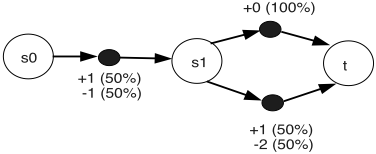
Example 1. Consider the MDP as in Figure 1: S = {s0, s1, t}, where t is the terminal state. The initial state s0 has one action, which leads to state s1, and the immediate reward is that with probability 0.5 it is +1, and otherwise -1. State s1 has two actions a and b, both lead to state t. The immediate reward of a is always 0, and that of b is that with probability 0.5 it is +1, and otherwise -2. Observe that for either fixed action a or b, Pr(X ≥ 0) = 0.5. In contrast, consider the policy π that at state s1, takes action a if the accumulated reward is +1, otherwise takes action b. Observe that Pr(Xπ ≥ 0) = 0.75, which shows that Πt,s is inferior to Πt,s,x .

Finally, we remark that adding extra information beyond the cumulative reward does not improve the performance for probabilistic goal MDP, as we will show in Section 5. The policies clasees Πt,s,x and Πh are therefore equivalent.

4 Complexity

In this section we show that in general, solving the probabilistic goal MDP is a computationally hard problem.

Theorem 2. The problemD(Π) is NP-hard, for Π equals to Πh , Πh,u, Πt,s , Πt,s,u, Πt,s,x or Πt,s,x,u .

Proof. We start with proving the result for Πt,s , by showing that we can reduce a well-known NP complete problem, KnapSack Problem (KSP), into a probabilistic goal MDP, and hence establish its NP-hardness. Recall that a KSP is the following problem. There are n items, 1 through n, each item i has a value vi and a weight wi. We can assume they are all non-negative integers. The KSP problem is to decide given two positive number W and V , whether there exists a I ⊆ [1 : n] such that

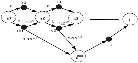
Given n, wi, vi, W and V , we construct the following MDP. Let T = n + 2. There are n + 2 states: S = {s1, · · · , sn, sbad , t}: s1 is the initial state and t is the terminal state. Each state si has two actions: if action a is taken, then the immediate reward is 0 and the next state will be si+1; if action b is taken, then the immediate reward is vi; furthermore, with probability 1/2wi the next state will be si+1 (respectively terminal state t if i = n) and otherwise the next state will be sbad . The state sbad has only one action which incurs an immediate reward -L ≜ -2 ∑ni=1 vi, and the next state will be t. See Figure 2.

Now consider the decision problem D(Πt,s ) with α = 1/2W . That is, to answer whether there exists π ∈ Πt,s such that

We now show that the answer to D(Πt,s ) is positive if and only if the answer to KSP is positive.

Suppose the answer to D(Πt,s ) is positive, i.e., there exists a policy π ∈ Πt,s such that

Define set I ′ as all i ∈ [1 : n] such that π takes b in si. Observe this implies that∑

Furthermore, due to the extreme large negative reward in sbad ,

which implies that

Thus, the answer to KSP is also positive.

Now suppose the answer to KSP is positive, i.e., there exists I ⊂ [1 : n] such that

Consider the following policy π′ of the MDP: take action b for all si where i ∈ I, and a otherwise. We have

Furthermore, when sbad is never reached, the cumulative reward is ∑i∈I vi ≥ V . Thus, we have that

i.e., the answer to D(Πt,s ) is also positive.

Thus, determining the answer to KSP is reduced to answering D(Πt,s ), the probabilistic goal MDP. Since the former is NP-complete, we conclude that probabilistic goal MDP is NP-hard.

Notice that in this example, Πt,s = Πt,s,x = Πh . Thus, NP-hardness for the decision problems with respect to these policy sets are established as well. Furthermore, Theorem 1 implies that D(Πh,u), D(Πt,s,u ), D(Πt,s,x,u ) are also NPhard.

5 Pseudo-polynomial algorithms

In the previous section we showed that it is of little hope that the probabilistic goal MDP can be solved in polynomial time. In this section we develop a pseudo-polynomial algorithm to handle this question. Recall that the running time of a pseudopolynomial algorithm is polynomial in the number of parameters and the size of the parameter, as opposed to polynomial algorithms whose running time is polynomial in the number of parameters and polylogarithmic in the size of the parameters.

5.1 Integer Reward

The main technique of our pseudo-polynomial algorithm is state augmentation. That is, we construct a new MDP in which the state space is the Cartesian product of the original state-space and the set of possible accumulated rewards. To better understand the algorithm, we first consider in this subsection a special case where the immediate reward is integervalued, i.e., R ⊂ Z. We show that the probabilistic goal MDP can be solved in time polynomial to |S|, |A| and K.

Theorem 3. Suppose that R ⊂ Z. In computational time polynomial in T , |S|, |A| and K, one can solve D(Πh,u ), i.e., determine the correctness of the following claim:

Similarly, in computational time polynomial to T , |S|, |A| and K, one can solve the probabilistic goal MDP, i.e., find π ∈ Πh,u that maximizes Pr(Xπ ≥ V ). Moreover, there exists an optimal solution to probabilistic goal MDP that belongs to Πt,s,x .

Proof. It suffices to show that an optimal solution to the probabilistic goal MDP

together with the optimal value Pr(Xπ∗ ≥ V ), can be obtained by solving an MDP with 2TK|S| states.

We construct a new MDP as follows: each state is a pair (s, C) where s ∈ S and C is an integer in [-TK, TK], and the initial state is (s0, 0). The action set for (s,C) is As, for all C. In time t, the transition between states is defined as follows:

That is, a transition to (s′ , C′ ) happens if in the original MDP, a transition to state s′ happens and the immediate reward is C′ -C. Notice that since the immediate reward of the original MDP is bounded in [-K,K] and there are only T stages, the accumulated reward of the original MDP is bounded in [-TK, TK]. The immediate-reward of the newMDP is zero except in the last stage, in which for states (s,C) with C ≥ V , a reward +1 is incurred.

It is easy to see that the solution to probabilistic goal MDP is equivalent to a policy that maximizes the expected reward for the new MDP. Note that there exists a deterministic, Markovian policy to the latter, then the probabilistic goal MDP has an optimal solution in Πt,s,x .

Theorem 3 leads to the following algorithm for solving probabilistic goal MDPs. Note that, not surprisingly, the proposed algorithm indeed parallels the standard algorithm (also pseudo-polynomial) solving KSP.

5.2 General Reward

In this section we relax the assumption that the reward is integer valued. We discretize the real-valued reward parameters to obtain a newMDP that approximates the original one. The new MDP is equivalent to an integer valued MDP, and hence can be solved in pseudo-polynomial time thanks to results

• Input: MDP < T, S,A,R, p, g >with R⊂ Z, V ∈ R.
• Output: π ∈ Πt,s,w that maximizes Pr(Xπ ≥ V ).
• Algorithm:
• Construct MDP with augmented state-space.
• Find a Markovian ˆπ∗ that maximizes the expected reward of the newMDP.
• Construct the policy of the original MDP as follows: the action taken at stage t, state s, with an accumulated reward C equals to ˆπt(s,C). Output the policy.

in Section 5.1. To show that such approximation is legitimate, we bound the performance gap that diminishes as the discretization becomes finer.

Theorem 4. There exists an algorithm, whose running time is polynomial in T , |S|, |A|, K and 1/ϵ, that finds a policy ˆπ, such that

Proof. Given an MDP 〈T, S,A,R, p, g〉, with K = maxr∈R |r|, and the grid size δ > 0, we can construct a new MDP < T , S, A, ˆR, p, ˆ g >, where ˆR = {iδ|i ∈ Z; -K/δ ≤ i ≤K/δ}, and

Observe that, by scaling the parameters, the new MDP is equivalent to an integer reward MDP whose reward parameters are bounded by K/δ. Hence the probabilistic goal MDP for the newMDP can be solved in time polynomial to T , |S|, |A|, K and 1/δ. Furthermore, as the next lemma shows, we can bound the error introduced by discretization.

Lemma 1. Let π be any policy, and ˆπ be the solution to the new probabilistic goal MDP. We have that

Proof. Fix t, s, a, by definition of ˆ gt, we have that for any c

Since the realization of reward parameters are independent, and there are T stages, this implies that

where ˆX denotes the (random) total reward for the newMDP. Since ˆπ maximizes Pr( ˆXπ ≥ V ), the lemma follows.

The theorem follows by setting δ = ϵ/T .

6 Chance ConstraintedMDPs

Thus far we investigated the case where we want to find a policy that maximizes the probability of achieving a predetermined target V . Another reasonable formulation is to treat this probability as a constraint: the decision maker may be interested in maximizing the expected reward while in the mean time ensures that the probability of achieving the target V is larger than a threshold. This leads to the Chance Constrained MDP (CC-MDP) formulation.

Problem 3 (Chance ConstrainedMDP). Given V ∈ Rand α ∈ (0, 1), find a policy π ∈ Πh,u that solves

Notice that checking the the feasibility of CC-MDP is equivalent to (NP-hard) D(πh,u ), which implies the NPhardness of CC-MDP. Nevertheless, similar as the probabilistic goal MDP, there exists a pseudo-polynomial algorithm that solves CC-MDP. However, in contrast to the probabilistic goal MDP, the optimal policy may be randomized. For succinctness we focus in this section the integer-reward case. Note that the general reward case can be approximated to arbitrary precision using discretization.

Theorem 5. Given an MDP such that R ∈ Z, V ∈ R, α ∈ [0, 1], the Chance Constrained MDP can be solved in a time polynomial in T, |S|, |A|,K. Furthermore, there exists an optimal solution π belongs to Πt,s,x,u.

Proof. Similar to the probabilistic goal MDP case, we construct a new MDP with augmented state space (s,C). The transition probability is defined in a same way as in the probabilistic goal MDP. However, we define the immediate reward as a pair (r1 , r2 ), both of which take non-zero values only at the last stage. In the last stage, if the state is (s,C), the first reward component is C and the second one is 1(C≥V ). Thus, observe that for a given policy π of this newMDP, the expected value of the first and the second component of the accumulated reward equals to the expected reward and probability of meeting the target of the original MDP, respectively. Thus, the chance constrained MDP is equivalent to find a policy of the second MDP that solves the following problem.

where X 1 π and X 2 π are the first and second component of the cumulative reward, respectively. Observe that Equation (1) is the well-studied constrained MDP formulation, which can be solved in polynomial time by converting it into a linear program [Altman, 1999]. It is also known that there exists a Markovian randomized optimal solution. Therefore, the chance constrained MDP can be solved in pseudo-polynomial time, and one optimal solution belongs to Πt,s,x,u.

We note that for CC-MDP , Πt,s,x is inferior to Πt,s,x,u , i.e., randomization may be necessary for optimal policies. This property is inherited from constrained MDPs and is due to the fact that we want to satisfy the probabilistic constraint while maximizing the expected reward.

7 Numerical Results

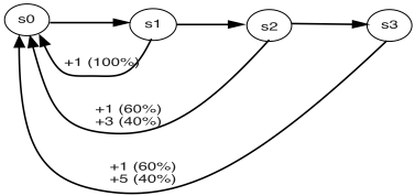
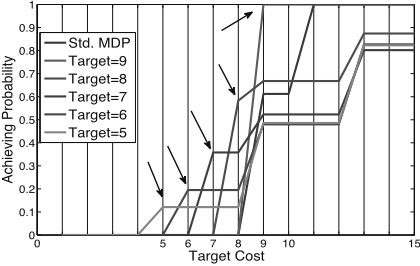
In this section we briefly report some simulation results that illustrate the performance of the proposed approach. We consider the following machine replacement example which is similar in spirit to [Delage and Mannor, 2010]. There are four possible states for a machine. The larger the state number, the worse the machine is. One can either replace the machine, which incurs a random cost, and the next state is s0, or "do nothing," with no cost, and the next state will be one state larger; see Figure 3. Fix T = 20. We compute the policy that minimizes the expected cost as in the standard MDP, and the policies that maximizes the probability that the cost is no larger than 5, 6, 7, 8, 9, respectively. For each policy, 1000 simulations are performed and the relative error is under 1%. We plot the performance of each policy in Figure 4: for a given x, the y-value is the frequency that the cumulative cost of a policy is smaller or equal to x. The simulation result clearly shows that each policy maximizes the chance of reaching its respective target.

8 Conclusion and Discussions

In this paper we proposed and investigated the probabilistic goal MDP model where the decision maker maximizes the probability that the cumulative reward of a policy is above a fixed target. We showed that while this formulation is NPhard, it can be solved in pseudo-polynomial time using state augmentation. We further discussed the chance constrained MDP formulation and showed it to be solvable in pseudopolynomial time.

The classical objective for MDP, considers only the expected cumulative reward, and hence may not capture the risk preference of the decision maker. The main thrust of this work is to address this shortcoming, with a decision criterion that is both intuitively appealing and also justified from a decision theory perspective, without sacrificing too much of the computational efficiency of the classical approach.

From an algorithmic perspective, the proposed algorithm for solving probabilistic MDPs may appear to be "easy" and not scale well, partly due to the fact that the problem is NPhard. However, we believe that by embedding the probabilistic MDP into a large scale MDP, it opens doors to use more scalable methods, in the spirit of approximate dynamic programming, that have been developed to handle large-scale MDPs, to approximately solve the probabilistic MDP. This is an interesting and important issue for future research.