
Context-Sensitive Diagnosis of Discrete-Event Systems
Proceedings of the Twenty-Second International Joint Conference on Artificial Intelligence. Pages 969-974.
https://doi.org/10.5591/978-1-57735-516-8/IJCAI11-167
© 2011 International Joint Conferences on Artificial Intelligence
Abstract
In a document network such as a citation network of scientific documents, web-logs etc., the content produced by authors exhibit their interest in certain topics. In addition some authors influence other authors' interests. In this work, we propose to model the influence of cited authors along with the interests of citing authors. Morover , we hypothesize that citations present in documents, the context surrounding the citation mention provides extra topical information about the cited authors. However, associating terms in the context to the cited authors remains an open problem. We propose novel document generation schemes that incorporate the context while simultaneously modeling the interests of citing authors and influence of the cited authors. Our experiments show significant improvements over baseline models for various evaluation criteria such as link prediction between document and cited author, and quantitatively explaining unseen text.
- [Aho et al., 2006] A. Aho, M.S. Lam, R. Sethi, and J.D. Ullman. Compilers -Principles, Techniques, and Tools. Addison-Wesley, Reading, MA, second edition, 2006.
- [Baroni et al., 1999] P. Baroni, G. Lamperti, P. Pogliano, and M. Zanella. Diagnosis of large active systems. Artificial Intelligence, 110(1):135-183, 1999.
- [Brand and Zafiropulo, 1983] D. Brand and P. Zafiropulo. On communicating finite-state machines. Journal of ACM, 30(2):323-342, 1983.
- [Cassandras and Lafortune, 1999] C.G. Cassandras and S. Lafortune. Introduction to Discrete Event Systems, volume 11 of The Kluwer International Series in Discrete Event Dynamic Systems. Kluwer Academic Publisher, Boston, MA, 1999.
- [Chomsky, 1956] N. Chomsky. Three models for the de- scription of language. Transactions on Information The- ory, 2(3):113-124, 1956.
- [Debouk et al., 2000] R. Debouk, S. Lafortune, and D. Teneketzis. Coordinated decentralized protocols for failure diagnosis of discrete-event systems. Jour- nal of Discrete Event Dynamic Systems: Theory and Applications, 10:33-86, 2000.
- [Jéron et al., 2006] T. Jéron, H. Marchand, S. Pinchinat, and M.O. Cordier. Supervision patterns in discrete event systems diagnosis. In Seventeenth International Work- shop on Principles of Diagnosis -DX'06, pages 117-124,
- Peñaranda de Duero, E, 2006.
- [Lamperti and Zanella, 2003] G. Lamperti and M. Zanella. Diagnosis of Active Systems -Principles and Techniques, volume 741 of The Kluwer International Series in Engi- neering and Computer Science. Kluwer Academic Pub- lisher, Dordrecht, NL, 2003.
- [Lamperti and Zanella, 2010] G. Lamperti and M. Zanella. Injecting semantics into diagnosis of discrete-event sys- tems. In 21st International Workshop on Principles of Di- agnosis -DX'10, pages 233-240, Portland, OR, 2010.
- [Pencolé and Cordier, 2005] Y. Pencolé and M.O. Cordier. A formal framework for the decentralized diagnosis of large scale discrete event systems and its application to telecom- munication networks. Artificial Intelligence, 164:121- 170, 2005.
- [Qiu and Kumar, 2006] W. Qiu and R. Kumar. Decentralized failure diagnosis of discrete event systems. IEEE Transac- tions on Systems, Man, and Cybernetics -Part A: Systems and Humans, 36(2):384-395, 2006.
- [Sampath et al., 1996] M. Sampath, R. Sengupta, S. Lafor- tune, K. Sinnamohideen, and D.C. Teneketzis. Failure di- agnosis using discrete-event models. IEEE Transactions on Control Systems Technology, 4(2):105-124, 1996.
- [Struss, 1997] P. Struss. Fundamentals of model-based diag- nosis of dynamic systems. In Fifteenth International Joint Conference on Artificial Intelligence -IJCAI'97, pages 480-485, Nagoya, J, 1997. IJCAI
- Morgan Kaufmann, S. Fran- cisco, CA.
References were extracted automatically from the PDF and may contain errors.
Full text extracted automatically from the PDF; figures, tables and equations may differ. The PDF is the version of record.
1 Introduction
A wide variety of techniques for diagnosis of discrete-event systems (DESs) [Cassandras and Lafortune, 1999] have been proposed in the last years, including [Baroni et al., 1999; Debouk et al., 2000; Lamperti and Zanella, 2003; Pencol´e and Cordier, 2005; Qiu and Kumar, 2006]. However, after the seminal work of [Sampath et al., 1996], the basic notions of fault and diagnosis have been remaining conceptually unchanged. Typically, a fault is associated with the occurrence of an event (or transition) at component level within the evolution of the system. Thus, diagnosing a DES amounts to uncovering the set of component faults occurring during the system evolution. The claim of this paper is that anchoring faults at component level is too restrictive an approach when complex DESs are involved.
2 Context-Sensitive Diagnosis
The topology of a complex DES is organized in a hierarchy, where the root corresponds to the whole system, leaves to components, and intermediate nodes to subsystems. Since in a DES faults are traditionally defined at component level, there is no possibility to provide a hierarchy of diagnoses adhering to the hierarchy of the system. Trivially, a sub-DES is faulty if and only if it includes a faulty component. We call this commonly-used approach context-free diagnosis. While context-free diagnosis may be adequate for simple systems, it is doomed to be unsatisfactory when applied to complex DESs. The hierarchical structure of a complex DES suggests to organize the diagnosis rules within a hierarchy that parallels the hierarchical structure of the DES: each subsystem has its proper set of diagnosis rules, which may or may not depend on the rules of inner subsystems. We call this alternative approach context-sensitive diagnosis.
The idea of context-sensitivity in diagnosis was inspired by the problem of (formal) language specification. The classical hierarchy proposed by [Chomsky, 1956] incorporates four types of generative grammars of growing expressiveness. Within the hierarchy, Type-2 and Type-1 grammars are means to specify the syntax of context-free and context-sensitive languages, respectively. For practical reasons, Type-2 grammars (in BNF notation) have become the standard for the specification of the syntax of programming languages. However, since, generally speaking, the syntax rules of programming languages depends on the context, production rules in BNF notation are unable to force all the syntax constraints of the language (for example: the list of actual parameters in a function call must match, in number and types, the list of formal parameters). In compilers, the check of these (contextsensitive) constraints are generally left to semantic analysis.
Loosely speaking, the idea of context-sensitivity can be profitably injected into diagnosis of DESs in three ways:
- SI The transition of a component is not considered either normal or faulty on its own: it depends on the context in which such a transition is triggered;
- SI The fault of a component is not necessarily ascribed to one transition: it can be the result of several transitions;
- SI Normal or faulty behavior of a subsystem is not necessarily determined by the normal or faulty behavior of its components (or inner subsystems).
Context-sensitive diagnosis is bound to seemingly contradictory but nonetheless possible results, called paradoxes.
2.1 Positive Paradox
The positive paradox states that a (sub)system may be normal despite the faulty behavior of a number of its components (or inner subsystems). Example 1 aims to clarify this assertion.
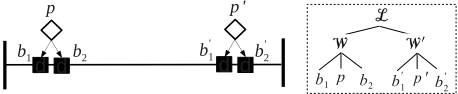
Example 1 Shown in the left of Fig. 1 is a simplified representation of a power transmission line. The line is protected on both sides by a redundant protection hardware, called W and W 0 , respectively, involving one protection and two breakers. For instance, W incorporates protection p, and breakers b1 and b2. When a lightening strikes the line, a short circuit may occur on the latter. The protection system is designed to open the breakers in order to isolate the line, which eventually causes the extinction of the short. To this end, when detecting a short circuit, a protection is expected to trigger both breakers to open. A protection is faulty when either it does not detect the short or, after the short detection, it does not trigger the breakers. A breaker is faulty when, after receiving the triggering command from the protection, it does not open. A minimal (non redundant) protection hardware would incorporate a single protection and a single breaker on each side of the line. Thus, when one of the two devices is faulty, the line cannot be isolated. By contrast, in the redundant protection hardware in Fig. 1, it suffices the normal behavior of the protection and of one breaker (for each side) to guarantee the isolation of the line. Consider the following two scenarios.
- In W, b1 is faulty, while p and b2 are normal. In W 0 , b 0 1 is faulty, while p 0 and b 0 2 are normal. The diagnosis is ı1 D fb1; b 0 1 g. Owing to redundancy, the behavior of the protected line is in fact normal, as the line is isolated, despite the faulty behavior of the two breakers.
- InW, b1 is faulty, while p and b2 are normal. InW 0 , p 0 is faulty, while b 0 1 and b 0 2 are normal. The diagnosis is ı2 D fb1; p 0 g. However, owing to p 0 , W 0 fails to open, causing the failure of the whole protected line.
Albeit the two diagnoses ı1 and ı2 differ in one component only (p 0 vs. b 0 1 ), the behavior of the protected line in the first scenario is normal, while it is faulty in the second one. The point is, the given diagnoses do not explicitly account for such a distinction. More generally, we can consider several subsystems of the protected line within an abstraction hierarchy, and require for each of them a diagnosis. Such a hierarchy is displayed in the right of Fig. 1, where L denotes the whole protected line. According to such a hierarchy, the diagnosis of the first scenario is fb1; b 0 1 g, while in the second scenario the diagnosis is fb1; p 0 ; W 0 ;Lg. Comparing the two diagnoses, we conclude that in the first scenario two components are faulty but their misbehavior is not propagated to higher subsystems. By contrast, in the second scenario, besides two faulty components (b1 and p 0 ), W 0 and L are faulty too. Þ
2.2 Negative Paradox
The negative paradox states that a (sub)system can be faulty despite the normal behavior of all its components (or inner subsystems). This is true also in systems other than DESs:
- SI A software system can be faulty even if all its software components are bug-free;
- SI A marriage may fail even if the behavior of each partner is unfailing on its own;
- SI A human society can be bound to dictatorship notwithstanding all its democratic institutions.
Example 2 instantiates the negative paradox to the referenced application-domain of power transmission networks.
Example 2 With reference to Fig. 1, the isolation of the line causes the extinction of the short circuit because the short is no longer fed by any current. This is why the protection system is designed to reconnect the line to the network once the short is extinguished (by closing breakers). Suppose now that, instead of a lightening, what causes the short is a tree fallen on the line. In this case, the reconnection of the line to the network presumably activates the short circuit again, as the tree is likely to be still on the line, thereby causing the line to be isolated anew (and, this time, permanently). Clearly, even assuming that the behavior of protections and breakers was normal, the behavior of the line is actually faulty. Þ
Coping with negative paradoxes is essential when the behavior of a complex DES cannot be foreseen at design-time (which is almost always the case for real DESs). To face this uncertainty, a set of constraints can be associated with the nodes of the DES hierarchy, aimed at intercepting relevant faulty-behavior. These constraints parallel the requirements of software systems, which need to be validated independently of the correct behavior of software components.
3 Active Systems
Active systems [Lamperti and Zanella, 2003] are a special class of asynchronous DESs. An active system is a network of components that are connected to one another through links. Each component is modeled as a communicating automaton [Brand and Zafiropulo, 1983], that reacts to events either coming from the external world or from neighboring components through links, and is endowed with input and output terminals. A transition from one state to another is triggered by an event ready at an input terminal: such a transition may generate other events at some output terminals of the same component. The mode in which a system can behave is constrained by its topology and the component models. The whole (even unbounded) set of evolutions of an active system is confined to a finite automaton representing the global model of the system. However, a strong assumption for diagnosis of active systems is the unavailability of the global model as, in real applications, the generation of the global model is impractical. The global model is intended for formal reasons only. The global model of a system˙, rooted at the initial state ˙0, is called the behavior space of ˙, written Bsp.˙; ˙0/. A history in Bsp.˙; ˙0/ is the list of component transitions marking the arcs of a path rooted in ˙0.
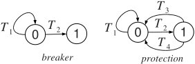
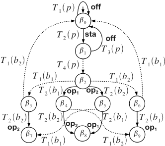
Example 3 With reference to Example 1, shown in Fig. 2 are the behavioral models of breaker and protection. The automaton of the breaker includes two states, 0 (closed) and 1 (open), and two transitions, which are both triggered by a tripping event sent by the protection. While T2 moves the breaker to open (correct behavior), T1 leaves the breaker stuck to closed. The automaton of the protection involves two states, 0 (idle) and 1 (awaken), and four transitions. Transition T2 is triggered by the occurrence of a short circuit on the line and awakes the protection. The actual tripping command to breakers is generated by T4. However, the protection may return to state 0 without sending any command to breakers (T3). The protection may even not be able to detect the short circuit (T1). Based on Fig. 1, the active systemW consists of protection p and breakers b1 and b2. The behavior space of W is outlined in Fig. 3, where arcs are marked by component transitions (labels in bold will be explained shortly). Þ
4 Diagnosis Problem
When reacting, an active system performs a list of transitions (history), that moves the system from the initial state to a final state. Since a number of such transitions are perceived to the observer as visible labels, such a history generates a list of labels, the trace of the history. A diagnosis problem } for a system ˙ is a 4-tuple
where ˙0 is the initial state of the system, V the viewer, O the observation, and R the ruler. The viewer maps each component transition to a label, thereby establishing how transitions are perceived. If the label is SI (null label) the transition is invisible, otherwise it is visible. The observation is a directed acyclic graph where nodes are marked by observable labels and arcs denote (partial) temporal precedence between nodes.
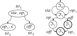
Example 4 With reference to system W defined in Example 3 and models in Fig. 2, we assume a viewer V with the following visible transitions and relevant labels: T2.b1/: op1, T2.b2/: op2, T1.p/: off, T2.p/: sta, T3.p/: off. Displayed in the left of Fig. 4 is an observation O relevant to viewer V, which is composed of three nodes and two arcs. Þ
An observation implicitly embodies several candidate traces, denoted kOk, each one obtained by picking up one label from each node of the observation without violating the temporal constraints imposed by arcs. Among such candidates is the (unknown) trace actually generated by the system history. For practical reasons, an index space of the observation O is generated, denoted Isp.O/. This is a deterministic automaton, where arcs are marked by the visible labels of O (SI aside). The regular language of Isp.O/ equals kOk, in other words, the set of paths in Isp.O/ equals the set of candidate traces of O.
Example 5 Shown in the right of Fig. 4 is the index space of observation O, where =3 and =4 are the final states. Þ
where D is the diagnosis domain, H the abstraction hierarchy, N the name space, F the fault space, and S the pattern specification. More specifically, the diagnosis domain D D fESC1; : : : ; ESCng is the set of subsystems of ˙ that are stated as relevant to the output of the diagnosis task. The abstraction hierarchy H defines a partition of each ESCi 2 D, i 2 Œ1 :: nc141, in terms of relevant subsystems, namely .ESCi ; fESCi1 ; : : : ; ESCini g/. The name space N is the set of identifiers used in S, while F DC2 N is the set of faults. Finally, the pattern specification S is a set of pairs .ESC; P/, where ESC 2 D and P D ŒP1; : : : ; Pkc141 is the pattern list, with each pattern Pi 2 P , Pi D .Ni ; Ei /, being the association between a name Ni 2 N and a regular expression Ei . The alphabet of Ei is defined as follows. Let .ESC; fESC1; : : : ; ESCmg/ 2 H. The alphabet A of ESC, where .ESC;P/ 2 S, is the union of the names relevant to patterns in P. The alphabet of a component C is the set of transitions relevant to the model of C. The alphabet A of Ei is defined as the union of the alphabets of the subsystems of ESC and the pattern names defined up to PiNUL1:
In other words, the regular expression Ei is defined on the pattern names relevant to the subsystems of ESC and those defined before Pi in the same pattern list P involving Ei . The plain form of Ei is the macro-substitution of each name in N by the corresponding regular expression. As such, the plain Ei is defined on the transitions of the components incorporated in ESC. The syntax of the regular expression on alphabet A is defined inductively as follows (assuming x and y to be regular expressions denoting languages L.x/ and L.y/):
- SI SI denotes the language fSIg (where SI is the null symbol);
- SI If a 2 A then a denotes fag;
- SI .x/ denotes L.x/ (parentheses are allowed as usual) ;
- SI x ‹ denotes L.x/ [ fSIg (optionality);
- SI x ETX denotes S 1 iD0 .L.x// i (iteration zero or more times);
- SI x C denotes S 1 iD1 .L.x// i (iteration one or more times);
- SI xy denotes L.x/L.y/ (concatenation);
- SI x j y denotes L.x/ [ L.y/ (alternative);
- SI x&y stands for .xy j yx/ (free concatenation).
| Subsystem ESC | Pattern list P |
|---|---|
| b1 | stc.b1/ D T1.b1/ |
| b2 | stc.b2/ D T1.b2/ |
| p | deaf .p/ D T1.p/ lazy.p/ D T2.p/T3.p/ fail.p/ D deaf .p/ j lazy.p/ |
| W | stc.b12/ D stc.b1/ & stc.b2/ nop.W/ D fail.p/ j stc.b12/ |
Example 6 A ruler R for system W defined in Example 3 is specified as follows. Diagnosis domain: D D fW; p; b1; b2g. The abstraction hierarchy H adheres to the tree outlined in the right of Fig. 1. N D fstc.b1/; stc.b2/; deaf .p/; lazy.p/, fail.p/; stc.b12/; nop.W/g. F D fstc.b1/; stc.b2/; deaf .p/, lazy.p/; nop.W/g. S is defined as shown in Table 1. For breakers b1 and b2, only one pattern is defined (stc, stuck to closed), involving transition T1. For protection p, three patterns are listed: deaf (p does not perceive the short circuit), lazy (although perceiving the short, p does not trip breakers), and fail (p is either deaf or lazy). For the protection hardware W, pattern stc.b12/ indicates both breakers stuck to closed. Finally, pattern nop (no operation) specifies when the protection hardware is faulty as a whole (when either p fails or both breakers are stuck to closed). Þ
5 Preprocessing
Once fault patterns are specified in terms of regular expressions, some (off-line) preprocessing on them is worthwhile to speed up the (on-line) diagnosis engine (which is in charge of solving the diagnosis problem). As known, [Aho et al., 2006], any regular expression can be automatically transformed into an equivalent deterministic finite automaton. Specifically, two steps are performed:
- For each pattern .Fi ;Ei / such that Fi 2 F , Ei is unfolded into its plain form (to include component transitions only) and an equivalent deterministic automaton Ai is generated, where final states are marked by Fi .
- The so-generated deterministic automata A1; : : : ;An within the same pattern list P (and, therefore, relevant to the same subsystem ESC) are merged to yield a new deterministic automaton called the pattern space of ESC , Pts.ESC /, where each final state S is marked by the set of faults associated with states identifying S. 1
The merging of automata in step 2 is performed as follows:
- SI Each automaton Ai is extended by inserting an empty transition from each non-initial state to the initial state.
- SI An empty transition is inserted from each initial state of each Ai to the initial state of each Aj , j ¤ i .
- SI The so-obtained nondeterministic automaton is transformed into an equivalent deterministic automaton, in fact Pts.ESC/, having as initial state the SI-closure of the set of initial states of A1; : : : ;An. Each final state S of Pts.ESC/ is marked by the union of faults associated with the states in S that are final in the corresponding Ai .
The rationale of the procedure above is that, during the reconstruction of the system behavior, the diagnosis engine is supposed to uncover several (possibly overlapping) fault patterns. This means that after the matching of any transition, the same fault pattern, or even a different one, may start.
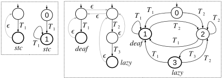
Example 7 Shown in Fig. 5 is the generation of the pattern space of a generic breaker b (left) and of protection p (right). Considering b, based on Table 1, fault pattern stc is defined as the single transition T1. The corresponding deterministic automaton generated by step 1 is represented by the two states and the arc marked by T1. Step 2 is performed by inserting the empty transition (gray arc). Pts.b/ is outlined next (second automaton in the figure). 2 The final node is marked by fault stc. Likewise, the generation of Pts.p/ is outlined in the right of Fig. 5. For space reasons, we have omitted the generation of Pts.W/ (whose final nodes are marked by fault nop). Þ
1 A state of the determinized automaton is identified by a subset of the states of the corresponding nondeterministic automaton.
2 States are identified by numbers, having however different meaning with respect to the homonym states of the models in Fig. 2.
6 Problem Solution
The solution of a diagnosis problem }.˙/ D .˙0; V; O; R/, written SOH.}.˙//, is a set of candidate diagnoses, where each candidate is a (possibly empty) set of faults. To define precisely SOH.}.˙//, we need to introduce a few notations. The trace of a history h of ˙ (based on viewer V) is written hŒVc141. The projection of h on a subsystem ESC, written hŒESCc141, is the sublist of transitions of h relevant to components in ESC. The language of a regular expression E is denoted by k E k.
Now, assume ruler R D .D; H; N ; F ; S/. The diagnosis of a history h based on R is:
That is, the diagnosis hŒRc141 is the set of faults F involved in a pattern list P of subsystem ESC, such that there exists a string e, in the language of the regular expression E relevant to F , that is a sublist of the projection on ESC of a history h. The solution of the diagnosis problem}.˙/ is:
That is, the solution of }.˙/ is the set of diagnoses of histories h whose trace, hŒVc141, is a candidate trace in O.
Example 8 Let }.W/ D .W0;V;O;R/ be the diagnosis problem for the protection hardware W defined in Example 3, where viewer V and observation O are defined in Example 4, while ruler R is specified in Example 6. The behavior space Bsp.W;W0/ is outlined in Fig. 3, where W0 D ˇ0 is the initial state and visible transitions are marked by relevant labels (in bold). The solution of }.˙/ can be determined based on eqn. (5). First, we have to select the histories in Bsp.W;W0/ whose trace is in kOk, in other words, whose trace is a path in the index space of O (Fig. 4). Of the six paths in Isp.O/ (from the initial state =0 to a final state (either =3 or =4), only Œsta; off c141 is consistent with Bsp.W;W0/, that is generated by history h D ŒT2.p/; T3.p/c141. Then, we have to determine the set ı of faults, where each fault F is associated with a regular expression E for subsystem ESC such that a path in k E k is contained in the projection of h on ESC. Based on the pattern specification in Table 1, of the five pattern names in F , namely stc.b1/, stc.b2/, deaf .p/, lazy.p/, and nop.W/, only lazy.p/ and nop.W/ meet such a condition. In fact, the only string in the regular expression of lazy.p/ equals hŒpc141 D h. Besides, unfolding the regular expression associated with nop.W/ yields the plain expression:
which includes hŒWc141 D h. Thus, based on eqn. (5), the solution of }.W/ is: SOH.}.W// D f lazy.p/; nop.W/ g. Þ
7 Diagnosis Engine
The diagnosis engine is required to take as input a diagnosis problem }.˙/ D .˙0;V;O;R/ and to output the solution SOH.}.˙//, as defined in eqn. (5). In doing so, it needs to reconstruct the behavior of ˙ that conforms to the observation, namely Bhv.}.˙//. We assume that the pattern spaces generated off-line by preprocessing (see Section 5) are available to the engine. Since a sort of pattern recognition is to be performed, states of Bhv.}.˙// will incorporate information not only on the observation but also on the pattern spaces in order to maintain the state of the matching.
Let B denote the set of states of Bsp.˙;˙0/, I the set of states of Isp.O/, and P D P1 STX P2 STX SOH SOH SOH STX Pn, where P1; : : : ;Pn are the set of states of pattern spaces Pts.ESC1/; : : : ; Pts.ESCn/, respectively. The behavior
is a deterministic automaton such that:
- SI S DC2 B STX I STX P is the set of states;
- SI S0 D .˙0; =0; P0/ is the initial state, where =0 is the initial state of Isp.O/, while P0 D .P10; : : : ; Pn0/ is the record of the initial states of Pts.ESC1/; : : : ; Pts.ESCn/;
- SI Sf D f.ˇ; =f; P/ j =f is final in Isp.O/g is the set of final states;
- SI T is the transition function: .ˇ; =; P/ T NUL! .ˇ 0 ; = 0 ; P 0 / 2 T , P D .P1; : : : ;Pn/, P 0 D .P 0 1 ; : : : ;P 0 n /, iff the following conditions hold:
- ˇ T NUL!ˇ 0 is a transition in Bsp.˙;˙0/; 3
- if T is invisible then = 0 D = else = 0 is the target state of transition = ` NUL! = 0 in Isp.O/, where ` is the label associated with T in V;
- P 0 D .P 0 1 ; : : : ;P 0 n / is such that 8i 2 Œ1 :: nc141, P 0 i is defined by the following rule:
As such, each state of Bhv.}.˙// is a triple involving a state of the behavior space, a state of the index space of O, and a record of pattern-space states. A transition marked by T is defined in Bhv.}.˙// iff a transition marked by T is defined between the corresponding states of the behavior space. The index = 0 of the new state differs from the index = in the old state only if T is visible (according to viewer V). Finally, considering P 0 in the new state, three cases are possible:
- (a) T is relevant to a component within ESC and there exists a transition in Pts.ESCi / exiting Pi , marked by T , and entering N Pi : P 0 i equals N Pi ;
- (b) T is relevant to a component within ESC and there not exists a transition in Pts.ESCi / exiting Pi and marked by T : P 0 i equals the initial state Pi 0 of Pts.ESCi /;
- (c) T is not relevant to a component within ESC: P 0 i equals Pi .
The rationale of case (b) is that the current pattern recognition fails to match any fault in ESCi , thereby causing the recognition process to start anew, at the initial state Pi 0. As to case (c), state Pi does not change because transition T is relevant to a component outside system ESCi , thereby being irrelevant to pattern recognition within Pts.ESCi /.
3 In practice, since Bsp.˙;˙0/ is assumed to be unavailable, it means that T is triggerable from state ˇ.
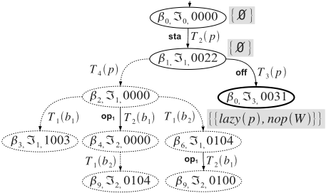
Example 9 Consider problem }.W/ D .W0;V;O;R/ defined in Example 8. Depicted in Fig. 6 is the relevant behavior Bhv.}.W// (node decoration will be explained shortly). According to the definition, the initial state is .ˇ0; =0; P0/, where =0 is the initial state of Isp.O/ (Fig. 4), while P0 D .0; 0; 0; 0/ is the record of the initial states of Pts.b1/, Pts.b1/, Pts.p/, and Pts.W/, respectively. Since the following conditions hold:
- SI Bsp.}.˙// (Fig. 3) includes a transition ˇ0 T2 NUL! ˇ1 which is visible via label sta of viewer V,
- SI A transition =0 sta NUL!=1 is included in Isp.O/,
- SI Transition T2.p/ is relevant neither to b1 nor to b2,
- SI P0 T2.p/ NULNULNULNUL! P2 is included in both Pts.p/ and Pts.W/,
a transition .ˇ0; =0; 0000/ T2.p/ NULNULNULNUL! .ˇ1; =1; 0022/ is generated in Bhv.}.W//. The construction of the behavior continues until no new node is generated by the application of the transition function. In Fig. 6, state .ˇ0; =3; 0031/ is final (in bold), as =3 is final in Isp.O/. The dashed part of the graph is inconsistent because it is not encompassed by any path from the initial state to a final state. Hence, it is eventually removed, leaving Bhv.}.W// with three states only. Þ
Once reconstructed the behavior Bhv.}.˙//, the diagnosis engine is required to generate the problem solution SOH.}.˙// defined in eqn. (5) by means of a sound and complete (possibly efficient) technique. This is carried out by decorating the nodes of the behavior with sets of faults as follows.
The fault set of P, written ıP, is the union of the faults associated with each state of P in the corresponding pattern space. We denote with SOH.S/ the set of sets of faults decorating state S in Bhv.}.˙//. Each state in Bhv.}.˙// is decorated with a set of sets of faults based on the following two rules:
- SI The initial state S0 D .˙0; =0; P0/ is first decorated by the singleton SOH.S0/ D fıP0 g.
- SI For each transition S T NUL!S 0 in Bhv.}.˙//, where S D .ˇ; =; P/, S 0 D .ˇ 0 ; = 0 ; P 0 /, the decoration of S 0 is defined by the following set-containment relationship:
The decoration algorithm starts by marking the initial state with a single diagnosis ıP0 including the set of faults associated with the initial state P0. Then, starting from the decoration of the initial state, it continuously applies the second rule for each transition exiting a state S whose decoration has changed. The rationale of (7) is as follows: if the current decoration of a state S of Bhv.}.˙// includes the set of faults ı and the reached state S 0 involves the record P 0 of patternspace states with associated faults ıP 0 , then the set of faults ı 0 associated with S 0 will be the extension of ı by ı 0 , as the latter is the set of faults relevant to the set of patterns recognized in state P 0 . The algorithm stops when the decoration becomes stable (the application of (7) will no longer produce any changes). Theorem 1 states how the actual solution of }.˙/ can be distilled from the decorated behavior.
Theorem 1 Let Bhv.}.˙// be the behavior of a diagnosis problem }.˙/. The union of the set of sets of faults decorating the final states of Bhv.}.˙// is the solution of }.˙/.
Proof. (Sketch) The proof is grounded on Lemma 1.1.
Lemma 1.1 Let EM be a path in Bhv.}.˙//, from the initial state to a final state. Let h be the list of component transitions marking the arcs of EM. Let ı be the union of the fault sets relevant to states of EM. Then, h is a history in Bsp.˙;˙0/ such that hŒVc141 2 kOk and hŒRc141 D ı.
Proof. The fact that h is a history in Bsp.˙;˙0/ such that hŒVc141 2 kOk derives from the mode in which fields ˇ and = are generated, specifically, from conditions 1 and 2 of transition-function of Bhv.}.˙//.
To prove hŒRc141 D ı, on the one hand, assume F 2 ı, that is, F 2 ıP, where .ˇ; =; P/ is a state in EM. As such, F is a fault associated with a (final) state of a pattern space Pts.ESC/. Since Pts.ESC/ is constructed by merging the deterministic automata relevant to the unfolded regular expressions involved in fault patterns, based on rule 3 of transition-function definition for Bhv.}.˙//, it means that a string e 2 k E k has been recognized, where .F;E/ is a fault pattern relevant to subsystem ESC, and e DC2 hŒESCc141. Hence, based on eqn. (4), F 2 hŒRc141.
On the other hand, assume F 2 hŒRc141, where h is a history in Bhv.}.˙//. Based on eqn. (4), F is the fault associated with an expression E, relevant to a subsystem ESC, such that there exists a string e in k E k that is a sublist of the projection of h on ESC. In other words, the projection of h on ESC contains a list of transitions that is a string relevant to the regular expression associated with F . Consider condition 3 in the definition of the transition function for Bhv.}.˙//, and the corresponding rule for the specification of P 0 . If T is relevant to a component in ESC then the state of the prefix space Pts.ESC/ in P changes either to the target state of the transition marked by T in Pts.ESC/ or to the initial state of Pts.ESC/, depending on whether or not such a transition exists in Pts.ESC/. Since the language of Pts.ESC/ contains the language of expression E (relevant to fault F), the string e will be matched within Pts.ESC/, where the state reached upon such recognition is marked (at least) by F . Hence, F 2 ı. Since F 2 ı , F 2 hŒRc141, we conclude hŒRc141 D ı. This terminates the proof of Lemma 1.1.
To prove Theorem 1, denoting with Sf a final state of Bhv.}.˙//, we have to show ı 2 SOH.Sf/ , ı 2 SOH.}.˙//.
Assume ı 2 SOH.Sf/. Based on the (two) decoration rules for Bhv.}.˙//, ı is obtained by (at least) one history h by extending the initial set of faults ıP0 by the set ıP 0 associated with each state S 0 D .ˇ 0 ; = 0 ; P 0 / encompassed by h. In other words, ı is the union of the fault sets relevant to states of h. Hence, by virtue of Lemma 1.1, ı D hŒRc141 and, based on eqn. (5), ı 2 SOH.}.˙//.
Assume ı 2 SOH.}.˙//. Based on eqn. (5), ı D hŒRc141. By virtue of Lemma 1.1, ı equals the union of the faults sets relevant to the states encompassed by h in Bhv.}.˙//. Following the same reasoning on the decoration rules above, this union is in fact an element of the decoration of the (final) state Sf of Bhv.}.˙// reached by h, hence, ı 2 SOH.Sf/. ETX
Example 10 With reference to the behavior Bhv.}.W// depicted in Fig. 6, the processing performed by the decoration algorithm is very simple, as the behavior is linear. 4 According to the first decoration rule, the initial state is marked by the singleton f;g, as ı0000 D ;. Applying the second rule, state .ˇ1; =1; 0022/ is decorated by f;g, as ı0022 D ;. For the final state Sf D .ˇ0; =3; 0031/, the decoration is the singleton fflazy.p/; nop.W/gg, which, based on Theorem 1, equals the solution SOH.}.W//, as confirmed by Example 8. Þ
8 RelatedWork
This paper is built upon [Lamperti and Zanella, 2010]. A related approach is proposed in [J´eron et al., 2006], where the notion of supervision pattern is introduced, which allows for a flexible specification of the diagnosis problem, and for an uniform solution of different classes of problems. However, three points are to be highlighted. First, supervision patterns are specified by automata. In this paper, instead, fault patterns are specified by regular expressions. Second, a supervision pattern specifies which system evolutions are to be considered as faulty (or, more generally, significant to the supervision process), based on specific occurrences of fault (and repair) events. In this paper, instead, a fault pattern specifies a (complex) fault within a system evolution. Finally, and more importantly, [J´eron et al., 2006] does not provide any hierarchical abstraction to diagnosis: since a diagnosis is an evolution identified by a supervision pattern, the notion of diagnosis invariably refers to the system as a whole. In this paper, instead, the interpretation of the system behavior is based on the abstraction hierarchy, where diagnosis rules are defined for each subsystem in the hierarchy.
9 Conclusion
Context-sensitive diagnosis is bound to enhance the expressive power of diagnosis of complex DESs. However, we do not consider the proposed notation for pattern specification as final: different formalisms can be envisaged to fit different classes of DESs. Maybe, the general approach is of benefit to diagnosis of complex systems other than DESs, from static systems to more general dynamic systems [Struss, 1997].
4 Generally speaking, based on eqn. (7), the decoration algorithm is required to visit the nodes of the behavior several times.
@inproceedings{ijcai2011p167,
  title     = {Context-Sensitive Diagnosis of Discrete-Event Systems},
  author    = {Lamperti, Gianfranco and Zanella, Marina},
  booktitle = {Proceedings of the Twenty-Second International Joint Conference on
               Artificial Intelligence, {IJCAI-11}},
  publisher = {AAAI Press/International Joint Conferences on Artificial Intelligence},
  editor    = {Toby Walsh},
  pages     = {969--974},
  year      = {2011},
  month     = {7},
  doi       = {10.5591/978-1-57735-516-8/IJCAI11-167},
  url       = {https://doi.org/10.5591/978-1-57735-516-8/IJCAI11-167},
}
TY - CPAPER TI - Context-Sensitive Diagnosis of Discrete-Event Systems AU - Lamperti, Gianfranco AU - Zanella, Marina T2 - Proceedings of the Twenty-Second International Joint Conference on Artificial Intelligence, IJCAI-11 PB - AAAI Press/International Joint Conferences on Artificial Intelligence PY - 2011 SP - 969 EP - 974 DO - 10.5591/978-1-57735-516-8/IJCAI11-167 UR - https://doi.org/10.5591/978-1-57735-516-8/IJCAI11-167 ER -Copied
Machine-readable versions of this paper, for tools and AI agents:





