Generalized Planning: Synthesizing Plans that Work for Multiple Environments

1 Introduction

Generalized planning, where a single plan works for multiple environments, has recently been drawing increasing attention in the AI community [Levesque, 2005; Srivastava et al., 2008; Bonet et al., 2009]. This form of planning has the advantage that if a generalized solution is found for a problem class, then solving any particular instance in the class only requires the execution of the generalized plan, which is extremely efficient since no search is needed in the execution.

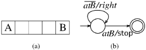
Consider the following example, which is a slightly simplified version of the problem proposed by Bonet et al.[2009]: Figure 1(a) shows a linear grid world, in which the robot, initially at cell A, can move left and right within the cells, and can observe whether it is at cell B. The goal is to make it at B. This problem has a simple sequential plan consisting of 4 consecutive right moves, but a more interesting solution is the one shown in Figure 1(b), which says "repeatedly move right, until atB is observed," in that it does not only solve this particular instance, but also any linear grid of arbitrary size.

Even in this simple example it is not immediately clear what it means that the plan "solves any linear grid." The difficulty comes from the heterogeneity of the problem instances. For this 1 × 5 example, we may have five boolean fluents to represent the grid, but for the 1 × 3 case, we may have only three. So the state space, among other things, is different across the problem instances. Then, what does it mean that the plan in Figure 1(b) is a valid solution for all of them?

Giuseppe De Giacomo

Dipartimento di Informatica e Sistemistica SAPIENZA Universit`a di Roma, Italy Via Ariosto 25, 00185 Roma, Italy

degiacomo@dis.uniroma1.it

To the best of our knowledge, the closest formal definition to planning of this type is given by Hu and Levesque [2010] in the situation calculus. However, they assume a fixed dynamic domain where the only uncertainty comes from the incomplete knowledge about the initial situation. As a result, the grid problems informally expressed above do not have a direct translation into their framework due to the variable number of propositions, although they can formulate a variant of this problem in terms of an unknown integer. Similarly, it is possible but indirect to understand this problem within the relational framework of Srivastava et al. [2011].

This raises the question whether one can find a general definition of generalized planning that is independent of any specific representation. In this paper, we give such a definition, making only minimal assumptions: we assume that a generalized plan must work on a set of deterministic environments, each with its own associated goal, whose state spaces may be completely unrelated, and which share only actions (used in plans), and observations (used as tests in plans).

We show that our definition is a natural extension of classical planning, conformant and conditional planning with deterministic actions. More importantly it captures and extends most generalized planning formalisms, including the ones mentioned above. We argue that our definition facilitates the research in this area, by presenting new insights into generalized planning in both finite and infinite environment sets.

For the finite case, we prove that generalized planning is always decidable and essentially EXPSPACE-complete. Notably, this is the same complexity as conformant and conditional planning under partial observability with deterministic actions. Our proof is constructive and gives us a sound, complete and complexity-wise optimal technique for generalized planning in finite environment sets. Interestingly, it turns out that the technique is based on compilation to classical planning, similar, in the spirit, to the methods used by Palacios and Geffner [2009] and Albore et al. [2009].

For the infinite case, we focus on planning for onedimensional (1d) problems, which is recursively enumerable when restricted to finite state controllers, in light of Hu and Levesque's finite verifiability theorem [2010]. We give a simpler reformulation of their finite verifiability theorem in our framework, and further show that concentrating on finite-state plans as generalized plans is actually not a restriction. Finally, we prove, somewhat surprisingly, that planning for this type of infinite environment sets is in fact decidable in EXPSPACE, assuming no sequence functions, and solvable by generalized planning in finite sets.

2 Generalized Planning

When dealing with planning, we need to consider two things: (i) the agent that executes the plan, and (ii) the environment in which the agent's plan is executed. These two parts are usually merged, together with the goal, in a so-called planning problem, but to highlight our notion of generalized planning as synthesizing a plan for multiple environments, we start by keeping them separated.

Agent. Plans are always executed by some agent, which has limitations on what it can observe and what actions it can perform. To formalize this intuition, we define an agent A as a tuple A = 〈Acts, Obs〉, where

• Acts is a set of actions the agent can perform, and
• Obs is a set of observations the agent can make.

To this, we may add constraints on the behavior of the agent, e.g., on the sequences of actions that it can perform, in order to further specify the agent's "capability." Such constraints could be in the form of transition systems, or more generally, temporal logic formulae over Acts and Obs. Being not a key element for this paper, we will not elaborate the details here.

Given an agent A = 〈Acts,Obs〉, a plan is a partial function p : Obs ∗ → Acts ∪ {stop}, where stop stands for plan termination. Such a partial function is required to be prefix closed: if p(o1, . . . on) is defined, then so is p(o1, . . . oi) for all i < n. This is a very general notion of plan that completely abstracts from syntactic or structural characterization of a plan representation. Such a notion of plan is common in automated process synthesis [Pnueli and Rosner, 1989] as well as in POMDP-based planning [Ghallab et al., 2004]. Notice that in order to define a plan, we only need the specification of the agent. In particular, we do not need any knowledge about the environment the agent acts in, so it is possible that the plan of an agent can be executed in multiple environments, which we define next.

Environment. An environment, in which an agent's plan is executed, is a tuple E = 〈Events, S, s0, δ〉, where

• Events is the set of all events in the environment;
• S is the internal state space of the environment;
• s0 ∈ S is its initial (internal) state;
• δ : S ×Events →S is the (partial) transition function.

As in classical planning we assume the environment is deterministic, i.e., there is only one initial state, and every event, if it happens in one state, may only take the environment to at most one single next state.

A trace on E is a sequence t = s0e1s1e2 · · · ensn, where s0 is the initial state of the environment E, and si = δ(si-1, ei) (and hence δ(si-1, ei) is defined) for all i = 1, . . . , n. We denote by last(t) the last state sn of t.

A goal for the environment E is a specification of desired traces on E. Note that (possibly by allowing for infinite traces) this definition is general enough to capture several types of goals, including temporally-extended and long-running (infinite) ones [Bacchus and Kabanza, 1998; De Giacomo and Vardi, 1999; Pralet et al., 2010]. For the purpose of this paper, however, we only concentrate on classical reachability goals, consisting in reaching one (anyone) of the desired states in G ⊆ S. We observe that in order to specify goals, we only require knowledge about the environment, and nothing on the agent that acts in such an environment.

Executing an agent's plan in an environment. In order to characterize the execution of an agent's plan in an environment, we need to know how the agent observations are related to the environment states, and the agent actions to the events happening in the environment. In particular, we need:

• An observation function obs : S → Obs, which determines how much of the environment the agent can observe for the purpose of plan execution, i.e., when selecting an action to perform, the states s1 and s2 cannot be distinguished by the agent if obs(s1) = obs(s2);
• An execution function exec : Acts → Events, which determines the events in the environment that the agent causes by doing its actions. This function enables separation between what the agent can do and what changes the environment may have. This is akin to Srivastava et al. [2011] where they distinguish between abstract actions of a plan and concrete actions in its execution. 1

Given the observation and execution functions, we can determine the execution of an agent A's plan p in the environment E. A run r of plan p in environment E is the trace trace(p) = s0e1s1e2 · · · ensn such that for all i = 1, . . . , n, ei = exec (p(obs(s0), . . . obs(si-1))). We call r complete if p(obs(s0), . . . obs(sn)) = stop and for all i < n, p(obs(s0), . . . obs(si)) ̸= stop. Notice that a plan, being deterministic, has at most one complete run in any given environment.

Basic planning problem. A (basic) planning problem P consists of an agent A = 〈Acts,Obs〉, an environment E = 〈Events, S, s0, δ〉 with a goal G for E, and related obs and exec functions. Formally a basic planning problem is a tuple P = 〈Acts, Obs, Events, S, s0, δ, G, obs, exec〉 where all the components are as above. A solution to a basic planning problem P is a plan p that generates a complete run r that fulfill the goal, i.e., such that last(r) ∈ G.

Generalized planning problem. A generalized planning problem P = {P1, P2, . . .} is a (finite or infinite) set of basic planning problems Pi, where all of the Pi = 〈Acts, Obs, Eventsi, Si, si0, δi, Gi, obsi, execi〉 share the same agent, i.e., Acts and Obs are kept fixed. A solution for a generalized planning problem P is a plan p, such that p is a solution for every Pi ∈ P. Intuitively, we require that the plan p for a fixed agent A = 〈Acts,Obs〉 achieves, on all of the environments Ei = 〈Eventsi, Si, si0, δi〉, their respective goals Gi. In other words, p is a solution for the generalized planning problem iff it generates, for each corresponding environment Ei, a complete run ri such that last(ri) ∈ Gi.

1 Notice that for simplicity we assume in this paper that an action of the agent corresponds to only one event in the environment (as in Srivastava et al.), but this could possibly be generalized. As an extreme case, an agent's action could as well correspond to an entire sequence, or a program, built from events. We leave exploring this issue for future research.

Example. With the definitions above, we can now formalize the grid example in the introduction.

Following Bonet et al. [2009], we can use one proposition for each cell in the grid, and define P = {P1, P2, · · · } with Pi = 〈Acts, Obs, Eventsi, Si, si0, δi, Gi, obsi, execi〉, where

• Acts = Eventsi = {left, right}, execi is identity,
• Obs = {atB, atB},
• Si = {p0, p0} × {p1, p1} × · · · × {pi, pi},
• si0 = 〈p0, p1, · · · , pi-1, pi〉,
• δi(〈p0, · · · , pl-1, pl, · · · , pi〉, left) = 〈p0, · · · , pl-1, pl, · · · , pi〉 for l = 1, · · · , i, and δi(〈p0, · · · , pl, pl+1, · · · , pi〉, right) = 〈p0, · · · , pl, pl+1, · · · , pi〉 for l = 0, · · · , i - 1,
• Gi = 〈p0, p1, · · · , pi-1, pi〉,
• obsi(s) = { atB if s = 〈p0, p1, · · · , pi-1, pi〉, atB otherwise.

Alternatively, we can appeal to an integer parameter, like in Hu and Levesque [2010], and get P = {P1, P2, · · · } with Pi = 〈Acts, Obs, Eventsi, Si, si0, δi, Gi, obsi, execi〉, where

• Acts = Eventsi = {left, right}, execi is identity,
• Obs = {atB, atB}, Si = {0, 1, · · · , i}, si0 = i,
• δi(n, left) = n+ 1 for n = 0, · · · , i - 1, and δi(n, right) = n - 1 for n = 1, · · · , i,
• Gi = {0},
• obsi(s) = { atB if s = 0, atB otherwise.

This variant is an instance of "one-dimensional planning problems" discussed later, so we can apply the results there to generate a plan despite the problem set being infinite.

Relationship to standard planning. Our definition of generalized planning is a direct generalization of standard forms of planning studied in the literature [Ghallab et al., 2004].

Classical planning. In a nutshell, classical planning is generalized planning for singleton environment sets. Indeed, classical planning can be formulated as P = {P}, where P = 〈Acts,Obs,Events, S, s0, δ,G, obs, exec〉, S and Events are finite, Acts = Events, exec is the identity function, Obs = {nil}, and obs(s) = nil for all s ∈ S.

It is well-known that if a plan exists, this can be computed by solving a reachability problem from the initial state s0 to some state s ∈ G. The resulting plan is simply a sequence of actions. We call such plan classical. Classical plans do not use the history of observations (which are all identical) except for its size: p(o1, · · · , on) = p(n).

Conditional planning. In our setting, conditional planning with partial observability, deterministic actions and unknown initial states can be formalized as P = {P1, · · · , PN}, where Pi = 〈Acts, Obs, Events, S, si0, δ, G, obs, exec〉 are identical except for the initial state si0. Here, S and Events are finite, Acts = Events and exec is the identity function. Notice that N can be at most the size of S, which happens when we know nothing about the initial state.

Conformant planning. We get conformant planning by further requiring that the agent has no observability, i.e., Obs = {nil} and obs(s) = nil for all s ∈ S.

Computational complexity. The computational complexity of classical planning is a direct consequence of the complexity of reachability in graphs, which is NLOGSPACEcomplete. Observe that we typically adopt a compact (i.e., logarithmic) representation of various elements of the planning problems, for example by using propositions to denote states and computing the transitions δ directly on such propositions. 2 In this case, assuming that the graph corresponding to the domain can be constructed on-the-fly, while doing the reachability test for the goal, and by Savitch's theorem NSPACE (f(n)) ⊆ DSPACE (f (n)2 ), we get that classical planning is PSPACE-complete [Bylander, 1994].

Conditional planning with partial observability, and conformant planning, with deterministic actions, require an exponential blow up of the states of the graph to be visited and as a result are PSPACE-complete in the size of Pi, and EXPSPACE-complete assuming a compact representation of Pi [Haslum and Jonsson, 1999; Rintanen, 2004]. Interestingly, this bound holds also for temporally extended and long running goals [De Giacomo and Vardi, 1999].

3 Finite Case

We now focus on generalized planning, assuming, like in the standard cases discussed above, a finite set of basic planning problems. We devise a sound and complete technique for generalized planning in this case, which gives us an EXPSPACE-complete characterization of the complexity of the problem (assuming a compact representation). Interestingly, the technique can be seen as a compilation of generalized planning into classical planning, in the spirit of Palacios and Geffner [2009] and Albore et al. [2009], although our focus is on understanding the computational complexity, instead of achieving maximal efficiency as they do.

Formally, the generalized planning problem we study in this section is of the form P = {P1, . . . , PN}, where each Pi = 〈Acts, Obs, Eventsi, Si, si0, δi, Gi, obsi, execi〉. Note that only Acts and Obs are shared across the various problems, and all other elements may differ.

To solve this problem, we use action vectors introduced by De Giacomo and Vardi [1999] in the context of conditional planning with partial observability for temporally-extended goals. We start by enumerating the (finite) basic problems from 1 to N. In this way, we can consider action vectors of the form ⃗a = 〈a1, . . . , aN〉, with one separate action ai for each problem Pi in the set P. Now, we consider sequences of action vectors. Notice that, if we project such an action vector sequence on component i we get a classical plan pi for problem Pi (i = 1, . . . ,N). However, in order for the sequences of action vectors to be considered a solution for the generalized planning problem P, we must require that, for each observation history o0 · · · ok such that both pi and pj are defined, pi(o0 · · · ok) = pj(o0 · · · ok), for i, j = 1, . . . ,N, i.e., if pi and pj have received the same observation so far, they must return the same action. To do so, we maintain an equivalence relation, which records whether pi and pj currently must return the same action. With this intuition in mind, we now show how to reduce the generalized planning problem P to a classical planning PP. Specifically, we construct PP = 〈ActsP , ObsP , EventsP , SP , sP0, δP , GP , obsP , execP 〉, with ActsP = EventsP , execP being the identity function, ObsP = {nil}, and obsP(s) = nil for all s ∈ S, as always for classical planning, and

2 We want to stress that assuming there are formalisms able to represent every planning problem compactly is not realistic. Indeed, the number of possible transition functions δ is |S||S| , while the number of transition functions distinguishable with O(log(|S|)) bits is 2O(log(|S|)) = |S|O(1) . In many cases, however, compact representations do exist, using planning languages like STRIPS or PDDL.

• ActsP = (Acts ∪ {stop})N , i.e., the set of N-vectors of actions fromActs plus a special stop action;
• SP = S1 ×· · ·×SN ×Eq ×Goals, where Eq is the set of equivalence relations on {1, . . . , N}, discussed above (the size of Eq is 2N 2 ), and Goals is all possible subsets of {1, . . . ,N}, which records for which problems the goal has been fulfilled (the size of Goals is 2N );
• sP0 = 〈s10, . . . , sN0, e0, g0〉, where the initial equivalence relation e0 = {〈i, j〉 | obsi(si0) = obsj(sj0)} records which basic planning problems get the same observations in their initial states, and g0 = {i | si0 ∈ Gi} lists the problems whose goals are satisfied initially.
• δP(〈s1, . . . , sN, e, g〉, 〈a1, . . . , aN〉) = 〈s′1 , . . . , s′N , e′ , g′ 〉, where
• 〈i, j〉 ∈ e then ai = aj, that is, if two plans have received the same observations so far, they must return the same action;
• if ai = stop, then si ∈ Gi, that is, the execution can legally terminate only in goal states;
• s′i = δi(si, execi(ai)), if i ̸∈ g′ , and s′i = si otherwise, that is, compute the next state for all Pi;
• e′ = {〈i, j〉 | 〈i, j〉 ∈ e and obsi(s′i ) = obsj(s′j )}, that is, update the equivalence relation eliminating from it those plan for which if the observation in the resulting state is different;
• g′ = {i | i ∈ g or ai = stop}, that is, update the list of problems whose goals have been achieved.
• GP = {〈s1, . . . , sN, e, gf〉 | gf = {1, . . . ,N}}, that is, we want to reach a state where all the goals Gi of the problems Pi have been fulfilled.

Theorem 1 (Soundness and Completeness). The generalized planning problem P has a solution iff the classical planning problem PP has one.

Note that the technique is constructive, and allows for extracting the generalized plan by unpacking the action vectors in the sequential plan. Such a generalized plan can easily be put into a more convenient tree-like finite-state form.

Next we turn to computational complexity. By building PP on-the-fly, we can check reachability of states in GP in a state space of size: O((Πi=1,...,N|Si|) × |Eq| × |Goals|)), where |Eq| = 2N 2 and |Goals| = 2N . This can be done by a nondeterministic algorithm needing O((Σi=1,...,N , log |Si|)+N 2 + N)) bits, which, assuming N and the maximum of the |Si| to be comparable, gives us a PSPACE upper bound (recall NPSPACE=PSPACE). A matching lower bound can be obtained considering that checking the non-emptiness of the intersection of N deterministic finite state automata over the same alphabet is PSPACE-complete [Garey and Johnson, 1979]. Such non-emptiness can be readily casted as a simplified generalized planning problem, where each component basic planning problem represents an automaton (using the goal as final states), and where there is no observation or distinction between actions and events. Finally, if we adopt a compact representation of the planning problems Pi, then generalized planning problem P becomes EXPSPACEcomplete, as conformant/conditional planning. So we have:

Theorem 2 (Complexity). Generalized planning in the finite case is PSPACE-complete (EXPSPACE-complete with respect to a compact representation).

4 Infinite Case

Next we move on to the general case, where the set of basic planning problems in the generalized planning problem is infinite, and briefly study its relationship to the recently proposed approaches to generalized planning [Bonet et al., 2009; Pralet et al., 2010; Hu and Levesque, 2010; Srivastava et al., 2011]. All these approaches aim at finding or characterizing generalized plans with a finite-state representation to solve classes of deterministic problems containing possibly infinitely many instances. Although they adopt different formalisms, they all fit into our definition of generalized planning which in facts inherits elements from all of them.

Bonet et al. [2009] synthesize a finite-state plan (controller) for a propositional problem, which often also solves "similar" problems, like the linear grid example in the introduction. They implicitly assume that the "similar" problems all share the same actions and observations, but formally not much else (although intuitively they share some structure). We built our framework directly on this intuition. To capture their intuition on generalization in our framework, we simply need to create a basic planning problem in the set for each of their problems. The same treatment also captures the goaloriented control problems of Pralet et al. [2010], although their safety-oriented and mixed problems require temporally extended goals in our framework as mentioned in Section 2.

Hu and Levesque [2010] formalize generalized planning in the situation calculus as a basic action theory with incomplete information about the initial situation. We share with them an approach that is well cut to get formal guarantees, though our representation is not based on specific logical formalisms. A natural translation from theirs involves defining a basic planning problem for each interpretation of their action theory.

Srivastava et al. [2008; 2011] learns a generalized plan for a relational domain (e.g., PDDL problems) from example solutions to selected problems. Due to varying objects, the problem instances in the domain may have different ground actions, but the plan may only have finitely many fixed actions. For this reason, "abstract actions" are used in their plan, i.e., actions whose arguments are not concrete objects in the domain, but instead what roles those objects must be in, where the role of an object is the set of all unary predicates it satisfies in the state. We share with them the distinction between actions performed by the agent and their execution in the environment. In particular, to capture their relational problems in our framework, we use their abstract actions as our agent actions, and create multiple basic planning problems with different exec functions to capture all possible concretizations of the abstract actions. The generalized planning problem is then the union of all basic planning problems obtained from each problem instance in their relational domain.

All three approaches above assume a finite-state representation for the plans. Recall that our plan is defined as a function Obs ∗ → Acts ∪ {stop}. In order to bridge this definition to what is commonly used in the literature, we call plan p : Obs ∗ → Acts ∪ {stop} to have a state form, if there is a set Q of plan states {q0, q1, · · · } and functions σ : Q×Obs →Q and α : Q×Obs →Acts, such that

By noting that we can use a plan state for each possible observation history, it is immediate to see that every generalized plan has a state form. However, we get a notable case when the set Q of plan states is finite, that is, p is a finite-state plan, which is indeed the form of generalized plan most used in the literature. Intuitively, the nodes in their graphical plan representation can be seen as the plan states, and the labeled edges represent the σ and α functions.

We close this discussion by arguing that our framework can facilitate research in generalized planning, not only by offering a common ground for existing approaches, but also by bringing more insight into the structure of the planning problems. As an example, we revisit Hu and Levesque's "onedimensional problems" [2010], and strengthen their results.

One-dimensional planning problems. Intuitively, onedimensional problems model cases where an unknown and unbounded number of entities exist, which require independent treatment to achieve the goal. Examples include treechopping [Levesque, 2005], delivery [Srivastava et al., 2008], trash-collection [Bonet et al., 2009], etc.

Here, for a cleaner presentation we adopt a slightly simplified version of one-dimensional problems wrt [Hu and Levesque, 2010], namely, we assume that all their finite fluents are binary, and there is no sequence function in the domain. Our results can be extended to deal with the original version as well, although it requires further elaboration.

Formally, a generalized problem P = {P0, P1, · · · } is onedimensional (simplified), or 1ds, if all

share the same Acts, Obs, Events, G and exec, and

1. si0 = 〈i,⃗b0〉;
2. if δi(〈n,⃗b〉, e) = 〈n- d,⃗b′ 〉 for n > 0, then d ∈ {0, 1}; furthermore, for all n′ > 0, δi(〈n′ ,⃗b〉, e) = 〈n′ - d,⃗b′ 〉;
3. G ⊆ {0}×{true, false}m;

Intuitively, n in the state tuple 〈n,⃗b〉 denotes the number of unprocessed entities, and ⃗b = 〈b1, · · · , bm〉 represent all the m boolean properties of those entities in the environment. Condition 5 above requires that states only differing in their non-zero integer part are observationally indistinguishable; 3 enforces that the objects can only be processed one-by-one and independently; 2 says that the initial states are similar except for the number of objects; finally, 4 indicates that the goal is achieved only when all objects are processed with certain properties satisfied.

The key result for one-dimensional problems is Hu and Levesque's Theorem 1 on the finite-verifiability [2010]. In our framework, we have the following analogous but notationally much simpler theorem.

Theorem 3. Given a 1ds problem P = {P0, P1, · · · } and a finite-state plan p with l plan states, if p is a plan for {P0, P1, · · · , PN}, where N = l · 2m + 1, with m being the number of booleans in each state, then p is a plan for P.

With our machinery in place, we can further strengthen this result by showing that finite-state plans are all we need for 1ds problems.

Theorem 4. If a 1ds generalized planning problem has a plan, then it has a finite-state plan. 3

This makes planning for 1ds problems at least recursively enumerable. To see this, we only need to enumerate and verify all finite-state plans with 1, 2, 3, · · · plan states, and the algorithm is guaranteed to terminate with a valid plan, as long as one exists. Actually, we can prove a much stronger result.

Theorem 5. A 1ds generalized problem P = {P0, P1, · · · } has a plan, if and only if the finite set P ′ = {P0, P1, · · · , PN} has a plan where N = 2m, with m being the number of boolean components in each state.

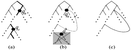
Proof sketch. The "only if" direction is trivial, so we focus on the "if" direction. Suppose we are given a plan p that solves P ′ . Without loss of generality, by Theorem 1, we can assume that p is a tree-like finite-state plan, as shown in Figure 2(a).

3 The proof follows the line of the one for Theorem 5 below, which can be seen as a refinement of this theorem.

Now consider the execution of p on the basic problem PN: if p decreases n from N to 0, then there must be at least N + 1 states with different integers in the run, but there are at most N = 2m boolean combinations, so at least two states in the run have identical boolean states. Let them be 〈N - u,⃗b∗ 〉 and 〈N -u-v,⃗b∗ 〉, respectively, and the corresponding plan states be qu and qv, as shown in the figure by the bold dots. Then, we redirect the incoming edge to qv into qu, and discard the sub-tree starting from qv, as shown in Figure 2(b). This gives us a finite-state plan p′ as shown in Figure 2(c), which is a generalized plan for P. To see this, for any basic planning problem Pk where k > N, the execution of p′ will enter qu in state 〈k-u,⃗b∗ 〉. If k-u > v, the execution of p′ will follow the loop and enter qu again in state 〈k-u-v,⃗b∗ 〉. This repeats until 〈v′ ,⃗b∗ 〉 is reached at qu for some v′ ≤ v. From there, the execution of p′ is guaranteed to terminate and achieve the goal, in the same way p runs on Pv′+u ∈ P ′ . This is due to the fact that v′ + u ≤ N, and that qu is reached in the very state 〈v′ ,⃗b∗ 〉 when running p on Pv′+u, from which p terminates and achieves the goal without ever reaching qv.

Theorem 5 gives us a sound and complete algorithm to solve 1ds problems: given problem P = {P0, P1, · · · }, we use any existing approach, possibly the reduction to classical planning introduced above, to find a generalized plan for the finite problem set {P0, P1, · · · , PN}. If a plan is found, we can construct a finite-state plan that works for P using the construction sketched above; otherwise, no plan exists for P.

In fact, from Theorem 5 considering that we can extract in polynomial time a looping plan from a tree-like plan according to the above construction, we get the following complexity upper bound (notice that 1ds problems use a compact problem representation by definition).

Theorem 6. Generalized planning for 1ds problems is EXPSPACE. 4

We close this section by observing that these results imply that the iterative procedure for planning in 1ds problems presented by Hu and Levesque [2009] is in fact sound, complete and terminating in 2EXPTIME (notice that the number of plan states is bounded by 2m). With these guarantees, such an iterative procedure, though not optimal with respect to computational complexity, can be quite effective in practice, since it explores simple solutions first.

5 Conclusion

We presented a framework that may serve the scientific community as a tool to increase the understanding of generalized planning and identify, among possibly other things, more general problem classes with interesting correctness and computational properties. We close the paper by noting that the framework can readily be extended to consider different kinds of goals, such as temporally-extended and long running ones. In fact, the results for the finite case can be extend to goals in linear temporal logic, by using techniques for automata on infinite strings, along the line of De Giacomo and Vardi [1999].

4 If sequence functions are introduced as in [Hu and Levesque, 2010], the same line of reasoning as above will give us a 2EXPTIME upper bound.

Acknowledgements. We thank Hector Geffner for interesting discussions that motivated our work, and we thank Hector Levesque, Sheila McIlraith, and the KR group at the University of Toronto, for feedback on how to improve the formalization. We acknowledge the support of EU Project FP7-ICT ACSI (257593).