
A Correctness Result for Reasoning about One-Dimensional Planning Problems
Proceedings of the Twenty-Second International Joint Conference on Artificial Intelligence. Pages 2638-2642.
https://doi.org/10.5591/978-1-57735-516-8/IJCAI11-439
© 2011 International Joint Conferences on Artificial Intelligence
Abstract
A plan with rich control structures like branches and loops can usually serve as a general solution that solves multiple planning instances in a domain. However, the correctness of such generalized plans is non-trivial to define and verify, especially when it comes to whether or not a plan works for all of the infinitely many instances of the problem. In this paper, we give a precise definition of a generalized plan representation called an FSA plan, with its semantics defined in the situation calculus. Based on this, we identify a class of infinite planning problems, which we call one-dimensional (1d), and prove a correctness result that 1d problems can be verified by finite means. We show that this theoretical result leads to an algorithm that does this verification practically, and a planner based on this verification algorithm efficiently generates provably correct plans for 1d problems.
- [Bonet et al., 2009] B. Bonet, H. Palacios, and H. Geffner. Automatic derivation of memoryless policies and finite- state controllers using classical planners. In Proc. of Intl. Conf. on Automated Planning and Scheduling, 2009.
- [Clarke et al., 1999] Edmund M. Clarke, Orna Grumberg, and Doron A. Peled. Model Checking. MIT Press, 1999.
- [Gelfond and Lifschitz, 1993] M. Gelfond and V Lifschitz. Representing actions and change by logic programs. Jour- nal of Logic Programming, pages 301-323, 1993.
- [Hu and Levesque, 2009] Y. Hu and H.J. Levesque. Planning with loops: Some new results. In ICAPS Workshop on Generalized Planning, 2009.
- [Levesque, 1996] H.J. Levesque. What is planning in the presence of sensing. In Proceedings of National Confer- ence on Artificial Intelligence, 1996.
- [Levesque, 2005] H.J. Levesque. Planning with loops. In Proc. of Intl. Joint Conf. on Artificial Intelligence, 2005.
- [Lin and Levesque, 1998] F. Lin and H.J. Levesque. What robots can do: robot programs and effective achievability. Artificial Intelligence, 1998.
- [Lin, 2008] F. Lin. Proving goal achievability. In Pro- ceedings of International Conference on the Principles of Knowledge Representation and Reasoning, 2008.
- [Magnusson and Doherty, 2008] M. Magnusson and P. Do- herty. Deductive planning with inductive loops. In Pro- ceedings of National Conference on Artificial Intelligence, 2008.
- [Manna and Waldinger, 1987] Z. Manna and R. Waldinger. How to clear a block: a theory of plans. Journal of Auto- mated Reasoning, 3(4):343-377, 1987.
- [McCarthy and Hayes, 1969] J. McCarthy and P.J. Hayes. Some philosophical problems from the standpoint of ar- tificial intelligence. Machine Intelligence, 1969.
- [Reiter, 2001] Raymond Reiter. Knowledge in Action: Logi- cal Foundations for Specifying and Implementing Dynam- ical Systems. MIT Press, 2001.
- [Scherl and Levesque, 2003] R. Scherl and H. Levesque. Knowledge, action, and the frame problem. Artificial In- telligence, 144, 2003.
- [Srivastava et al., 2008] S. Srivastava, N. Immerman, and S. Zilberstein. Learning generalized plans using abstract counting. In Proceedings of National Conference on Arti- ficial Intelligence, 2008.
- [Thielscher, 1998] M. Thielscher. Introduction to the flu- ent calculus. Electronic Transactions on Artificial Intel- ligence, 2(3-4):179-192, 1998.
- [Winner and Veloso, 2007] E. Winner and M. Veloso. LoopDISTILL: Learning domain-specific planners from example plans. In Proceedings of ICAPS-07 Workshop on AI Planning and Learning, 2007.
References were extracted automatically from the PDF and may contain errors.
Full text extracted automatically from the PDF; figures, tables and equations may differ. The PDF is the version of record.
Introduction
Planning with rich control structures like branches and loops is drawing increasing attention from the AI community [Manna and Waldinger, 1987; Levesque, 2005; Srivastava et al., 2008]. One advantage of the resulting generalized plan is that the same plan can work in different initial states with very large numbers of objects.
For example, suppose we have the following variant of the logistics problem: There are a number of objects at their source locations (office or home), and the goal is to move them all to their destinations with a truck. The available actions include moving the truck to a location, loading and unloading an object, finding the source and destination locations of an object, and checking whether all objects have been processed. Then, intuitively, the plan in Figure 1 achieves the goal no matter how many objects there are.
Unfortunately, it is not easy to see formally why this plan is correct for this problem. We need a formal definition of a plan representation and we must be precise about what it means for such a plan to be correct for all of the infinitely many possible objects and source-destination combinations.
∗This is a reduced version of the paper with the same name from KR-10. More details and proofs of theorems can be found there.
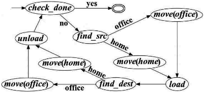
In this paper, we propose a solution to these in terms of a Finite State Automaton plan (FSA plan), a generalized plan representation inspired by and shown more expressive than robot programs [Levesque, 1996]. The semantics of FSA plans is declaratively defined in the situation calculus, so we have a foundation to analyze planning problems, plans, and their correctness. This notion of correctness, although precise and general, has the disadvantage that it uses second-order logic and is thus intractable in general. The intractability is inevitable, since FSA plans, like robot programs, are Turing complete in sufficiently expressive action domains [Lin and Levesque, 1998].
However, for restricted action domains, we can do much better. A number of real-world problems involve independently processing an unbounded number of objects: delivering packages according to their shipping labels (as in the logistics example above), pushing the buttons on a safe according to the digits of a combination, keeping or discarding eggs according to their smell, etc. In this paper, we identify a class of planning problems, which we call one-dimensional or 1d, that includes these, based on the shape of their action theory. We introduce a verification procedure, which we prove is correct for all 1d problems. We also present empirical evidence that a planner based on this verification procedure efficiently generates provably correct plans on planning problems that appear to be beyond the algorithmic reach of other planners.
Problem and Plan Representation
In order to represent and reason about the planning problem sketched above, we need a formal action language. In this paper, we appeal to the situation calculus, although the results introduced here could be adapted to other formalisms like A [Gelfond and Lifschitz, 1993], and the fluent calculus [Thielscher, 1998].
The situation calculus is a first-order, multi-sorted logical language with limited second-order features for representing and reasoning about dynamical environments [McCarthy and Hayes, 1969; Reiter, 2001]. Objects in the domain of the logic are of three disjoint sorts: situation for situations, action for actions and object for everything else. The only situation constant S0 denotes the initial situation where no action has yet occurred, and do(a, s) represents the situation after performing action a in situation s. We use do([a1, · · · , an], s) as an abbreviation for do(an, do(· · · , do(a1, s))). Functions (relations) whose value may vary from situation to situation are called functional (relational) fluents, and denoted by a function (relation) whose last argument is a situation term. Functions and relations whose value do not change across situations are called rigids. Without loss of generality, we assume that all fluents are functional. The special relation Poss(a, s) states that action a is executable in situation s, and the function SR(a, s) indicates the sensing result of a when performed in s. The latter is introduced by Scherl and Levesque (2003) to accommodate knowledge and sensing in the situation calculus. We assume that ordinary actions, not intended for sensing purposes, simply return a fixed value (ok). A formula φ is uniform in s if it does not mention Poss, SR, or any situation term other than s. We call a fluent formula φ with all situation arguments eliminated a situationsuppressed formula, and use φ[s] to denote the uniform formula with all situation arguments restored with term s.
The dynamics of a planning problem is formalized by a basic action theory (BAT) of the form
where
- FA is a set of domain-independent axioms defining the legal situations [Reiter, 2001].
- Σpre is a set of action precondition axioms, one for each action symbol of the form Poss(A(⃗x), s) ≡ ΠA(⃗x, s).
- Σpost is a set of successor-state axioms, one for each fluent f of the form f(⃗x, do(a, s))=y ≡ Φf (⃗x, a, y, s).
- Σsr is a set of sensing result axioms, one for each sensing action of the form SR(A(⃗x), s)=r ≡ ΘA(⃗x, r, s).
- Σ0 is the initial knowledge base stating facts about S0.
- Σuna is a set of unique names axioms for actions.
Figure 2 shows a complete specification for the logistic problem above as a BAT. 1 There are four fluents, loc (the location of the truck), loaded (the loading status of the truck), parcels left (the number of parcels remaining to be delivered), and misplaced (whether any processed object has been misplaced). The initial value of parcels left is non-negative but unknown. There is a sensing action check done that tells
1 We omit the foundational axioms FA, the unique names axioms Σuna, and any domain closure axiom for objects (as will be introduced in Definition 6 below).
Precondition Axioms:
Poss(move(x), s) ≡ TRUE Poss(load, s) ≡ loc(s) = source(parcels left(s)) ∧ loaded(s) = FALSE Poss(unload, s) ≡ loaded(s) = TRUE Poss(find src, s) ≡ parcels left(s) ̸= 0 Poss(find dest, s) ≡ parcels left(s) ̸= 0 Poss(check done, s) ≡ TRUE Successor State Axioms: loc(do(a, s)) = x ≡ ∃y. x = y ∧ a = move(y) ∨ x = loc(s) ∧ a ̸= move(y) misplaced(do(a, s)) = x ≡ x = TRUE ∧ a = unload ∧ loc(s) ̸= dest(parcels left(s)) ∨ x = misplaced(s) ∧ (a ̸= unload ∨ loc(s) = dest(parcels left(s))) loaded(do(a, s)) = x ≡ x = TRUE ∧ a = load ∨ x = FALSE ∧ a = unload ∨ x = loaded(s) ∧ a ̸= load ∧ a ̸= unload parcels left(do(a, s)) = x ≡ x = parcels left(s) -1 ∧ a = unload ∨ x = parcels left(s) ∧ a ̸= unload Sensing Result Axioms: SR(find src, s) = r ≡ source(parcels left(s)) = r SR(find dest, s) = r ≡ dest(parcels left(s)) = r SR(check done, s) = r ≡ r = yes ∧ parcels left(s) = 0 ∨ r = no ∧ parcels left(s) ̸= 0 SR(move(x), s) = r ≡ r = ok SR(load, s) = r ≡ r = ok SR(unload, s) = r ≡ r = ok Initial Situation Axiom: ∀n. (source(n) = home ∨ source(n) = office) ∧ ∀n. (dest(n) = home ∨ dest(n) = office) ∧ loc(S0) = home ∧ loaded(S0) = FALSE ∧ parcels left(S0) ≥ 0 ∧misplaced(S0) = FALSE Goal Condition:Figure 2: Axiomatization of logistic in the situation calculus
whether or not all parcels have been processed. In addition to the four fluents, we assume there are two rigid functions, source and dest that provide the shipping label for each object. For example, dest(7) = home would mean that the destination of the 7th object is home. The values of these functions is not specified, but the sensing action find src returns the source for the current object (according to parcels left), and similarly for find dest.
Given the dynamics, the planning task is to find a plan that is executable in the given environment, and whose execution achieves some desired goal. Here, we only consider planning problems with final-state goals, defined as follows:
Definition 1 (The Planning Problem). A planning problem is a pair 〈D, G〉, where D is a basic action theory, and G is a situation-suppressed formula in the situation calculus.
In the case of logistic, the goal G is to make parcels left be 0 while keeping misplaced as FALSE. Since the number of parcels and their sources and destinations are left open, this planning problem is not soluble with a sequential plan. We need a more general plan representation with branches and loops to handle the contingencies.
One candidate representation is Levesque's robot programs [Levesque, 1996]. Recently, Hu and Levesque (2009) proposed an alternative representation called the FSA plan, and showed that it is more general than robot programs, in that all robot programs have an FSA plan representation but not vice versa. Moreover, they also presented a planning algorithm with this representation, which greatly outperforms the robot-program based KPLANNER [Levesque, 2005]. As a result, we appeal to FSA plans in this paper.
Definition 2 (FSA Plan [Hu and Levesque, 2009]).
An FSA plan is a tuple 〈Q, γ, δ, Q0, QF 〉, where
- Q is a finite set of program states;
- Q0 ∈ Q is an initial program state;
- QF ∈ Q is a final program state;
- γ : Q→ A is a function, where Q= Q \ {QF } and A is the set of primitive actions;
- δ : Q×R → Q is a function, where R is the set of sensing results, that specifies the program state to transition to for each non-final state and valid sensing result for the associated action.
An example of an FSA plan (shown as a graph) appears in Figure 1. The execution of an FSA plan starts from q = Q0, and executes the action γ(q) associated with program state q. On observing sensing result r, it transitions to the new program state δ(q, r). This repeats until QF is reached.
In order to represent FSA plans in the situation calculus, we assume that there is a sub-sort of object called programstate, with Q0 and QF being two constants of this sort, and two rigid function symbols γ and δ. We use a set of sentences FSA to axiomatize the plan:
Definition 3. FSA is a set of axioms consisting of
- Domain closure axiom for program states (∀q). {q = Q0 ∨ q = Q1 ∨ · · · ∨ q = Qn ∨ q = QF };
- Unique names axioms for program states
- Action association axioms, one for each program state other than QF , of the form γ(Q) = A
- Transition axioms of the form δ(Q, R) = Q′
To capture the desired execution semantics, we introduce a transition relation T ⋆ (q1, s1, q2, s2), which intuitively means that from program state q1 and situation s1, the FSA plan will reach q2 and s2 at some point during the execution. The formal definition is given in Definition 4.
Definition 4. We use T ⋆ (q1, s1, q2, s2) as abbreviation for (∀T).{. . . ⊃ T(q1, s1, q2, s2)}, where the ellipsis is the conjunction of the universal closure of the following:
- T(q, s, q, s)
- T(q, s, q′′ , s′′ ) ∧ T(q′′ , s′′ , q′ , s′ ) ⊃ T(q, s, q′ , s′ )
- γ(q) = a ∧ Poss(a, s) ∧ SR(a, s) = r ∧ δ(q, r) = q′ ⊃ T (q, s, q′ , do(a, s))
Notice that this definition uses second-order quantification to ensure that T ⋆ is the least predicate satisfying the three properties above. This essentially constrains the set of tuples satisfying T ⋆ to be the reflexive transitive closure of the one-step transitions in the FSA plan.
With this transition relation, we can now characterize the correctness of FSA plans as follows.
Definition 5 (Plan correctness). Given a planning problem 〈D, G〉, a plan axiomatized by FSA is correct iff
The definition essentially says that for an FSA plan to be correct, it must guarantee that for any model of D, the execution of the FSA plan will reach the final state QF , and the goal is satisfied in the corresponding situation s. (In the case of logistic, a plan needs to work for any initial value of parcels left and any value for the functions source and dest.)
This criterion of correctness is general and concise, but its second-order quantification and the potential existence of infinitely many models make it less useful algorithmically. Partly for this reason, existing iterative planners based on a similar representation, like KPLANNER [Levesque, 2005] and FSAPLANNER [Hu and Levesque, 2009], only come with a very weak correctness guarantee: although the generated plan tends to work for all problems in the domain, only certain instances can be proven correct. It is thus interesting to ask whether we can generate provably correct plans for restricted classes of planning problems. The rest of this paper gives a positive answer to this question.
One-Dimensional Planning Problems
The major goal of this paper is to identify a class of planning problems that has a complete procedure to reason about the correctness of solution FSA plans. In this section, we define the class of 1d planning problems, which is derived from the more restricted finite problems.
Definition 6. A planning problem 〈D,G〉 is finite if D does not contain any predicate symbol other than Poss and equality, and the sort object has a domain closure axiom
Intuitively, a finite problem has finitely many objects in the domain. Therefore, the number of ground fluents as well as their range is finite.
A 1d problem is like a finite problem except that there is a special distinguished fluent (called the planning parameter) that takes value from a new sort natural number, there is a finite set of distinguished actions (called the decreasing actions) which decrement the planning parameter, and some of the functions (called sequence functions) have an index argument of sort natural number. 2 In the case of the logistic example, the planning parameter is parcels left, the decreasing action is unload, and the sequence functions are source and dest. The idea of a 1d planning problem is that the basic action theory is restricted in how it can use the planning parameter and sequence functions, as follows:
Definition 7. A planning problem 〈D′ ,G′ 〉 is 1d with respect to an integer-valued fluent p, if there is a finite problem 〈D,G〉 whose functions include fluent f0 and rigids f1, · · · , fm, andwhose actions includeA1, · · · ,Ad, such that 〈D′ ,G′ 〉 is derived from 〈D,G〉 as follows:
- Replace the fluent f0 with a planning parameter p:
where Dec(a) stands for (a = A1 ∨ · · · ∨ a = Ad);
- (b) replace all atomic formulas involving the term f0(s) in Π, Φ, Θ and G[s] by p(s) = 0, where s is the free situation variable in those formulas;
- (c) remove all atomic formulas mentioning f0(S0) in Σ0, and add p(S0) ≥ 0 instead.
- Replace the rigids f1, · · · , fm with sequence functions h1, · · · , hm:
- (a) replace all terms fi in Π, Φ, Θ and G[s] by hi(p(s)), where s is the free variable as above;
- (b) replace all fi in Σ0 with hi(n), where n is a universally quantified variable of sort natural number.
Observe that in a 1d problem, the occurrence of the integer planning parameter is limited to its own successor state axiom, in Σ0, and as an argument to a sequence function. Any other use of it is to test whether it is 0. Similarly, we can only apply a sequence function to the current object as determined by the planning parameter (other than in Σ0 where we must quantify over all natural numbers). This ensures that the objects can be accessed sequentially in descending order, and that they do not interact with one another. It is not hard to see that logistic conforms to these requirements.
Main Theorems
Given a planning problem and a candidate plan, an important reasoning task is to decide whether the plan is guaranteed to achieve the goal according to the action theory. In a 1d setting, we need to ensure that the plan achieves the goal no matter what values the planning parameter p and the sequence functions hi take. Unfortunately, there are infinitely many values that need to be taken into account.
In this section, we consider a correctness result of the following form: if we can prove that a plan is correct under the assumption that p(S0) ≤ N (for a constant N that we calculate), it will follow that the plan is also correct without this assumption. In other words, correctness of the plan for initial values of p up to N will be sufficient.
2 For simplicity, we assume in this paper that all sequence functions are rigid, but it is not hard to prove that the definitions and theorems work for sequence fluents as well.
The first theorem we can prove is the following:
Theorem 1. Suppose 〈D,G〉 is a 1d planning problem with planning parameter p, and that D contains FSA axioms for some plan. Let N0 = 2 + k0 · lm, where k0 is the number of decreasing program states in the FSA plan, m is the total number of finite and sequence functions, and l is the total number of values that they can take. Then we have:
What the proof does is to show that despite the fact that the value of the planning parameter is not bounded, the number of situations that can be distinguished in a 1d BAT is bounded. So if a plan were to fail to achieve the goal in a model where p(S0) > N0, then according to the BAT, it would also fail in a model where p(S0) ≤ N0.
The bound N0 in this theorem is exponential in the number of ground functions, however. It can therefore can be extremely large even for relatively simple action theories.
To obtain a more practical bound in a similar vein, we introduce another theorem, where we do not declaratively specify the bound, but instead only spell out the necessary condition for an integer Nt to be a valid bound.
Theorem 2. Suppose 〈D,G〉 is a 1d planning problem with planning parameter p, and that D contains FSA axioms for some plan. Let Seen(q, s) be the abbreviation for
where the first conjunction is over the finite fluents f, and the second over sequence functions h. Suppose Nt > 0 satisfies
Then we have the following:
Intuitively, the Nt here has to be large enough so that a similar situation to the one that decrements the planning parameter from 1 to 0 occurs earlier in the execution trace.
Experimental Results
Given an FSA plan for a 1d planning problem, Theorems 1 and 2 suggest two algorithms to verify its correctness, which can then be used for plan generation.
Plan verification
To utilize the idea in Theorem 1, we only need to execute the FSA plan for p(S0) = 0, 1, · · · ,N0. If the goal is achieved in all cases, then the FSA plan is correct in general, according to the theorem, and otherwise, it is incorrect. However, when the bound is large, this algorithm becomes impractical, since the number of possible initial worlds is exponential in the planning parameter. In the logistic example, for instance, each parcel has four possible source-destination combinations, so if we consider a problem containing 514 parcels (see the bounds for logistic below), the total number of possible combinations would be 4514 .
Fortunately, the bound N0 is a loose, worst-case estimate, and Theorem 2 suggests a better algorithm. We execute the FSA plan starting from p(S0) = 0, 1, 2, · · · . In each execution, whenever the planning parameter p decreases from 1 to 0, we record the program state, as well as the value of all finite and sequence functions in a table. If for some Nt, the execution for p(S0) = Nt does not add any new row into the table, then this Nt satisfies the criterion of Theorem 2, and thus the plan is guaranteed to be correct in general. If the FSA plan fails before reaching such an Nt, then it is incorrect. Notice that when the plan is correct, this algorithm will terminate, since if we reach N0, it is guaranteed correct by Theorem 1.
Plan generation
With the complete verification algorithms in hand, we can now generate plans that are correct for 1d planning problems. This is done by slightly modifying FSAPLANNER introduced by Hu and Levesque (2009).
The FSAPLANNER works by alternating between a generation and a testing phase: it generates plans for values of the planning parameter up to a lower bound, and then tests the resulting candidate plans for a higher value of the planning parameter. Although this appears to work for many applications, it has at least two serious problems: (1) the lower and higher bounds must be set by hand and (2) the only formal guarantee is that the plan works for the given values.
The verification algorithms proposed above resolve both of these problems. The idea is to replace the test phase of FSAPLANNER by this verification. Then whenever a plan passes the testing phase, it is guaranteed to be correct. Notice that in both cases, the bounds N0 and Nt can be obtained mechanically from the planning problem itself without manual intervention. The former only depends on the number of fluents and constants that appear in Σ0 and Σpost, whereas the latter is identified by table saturation.
We ran several experiments with variants of FSAPLANNER on four example domains: treechop, variegg, safe and logistic. (The first two are adapted from [Levesque, 2005].)
treechop: The goal is to chop down a tree, and put away the axe. The number of chops needed to fell the tree is unknown, but a look action tells whether the tree is up or down. Intuitively, a solution involves first look and then chop whenever up is sensed. This repeats until down is sensed, in which case we store the axe, and are done.
variegg: The goal is to get enough good eggs in the bowl from a sequence of eggs, each of which may be either good or bad, in order to make an omelette. A sensing action check bowl tests if there are enough eggs in the bowl, and another smell dish tests whether the egg in the dish is good or bad. Other actions include breaking an egg in the sequence to the dish, moving the egg from dish to bowl and dumping the dish.
| Problem | treechop | variegg | safe | logistic |
|---|---|---|---|---|
| Nman Time | 100 | 6 | 4 | 5 |
| (secs) | 0.1 | 0.12 | 0.09 | 3.93 |
| N0 | 18 | 345 | 4098 | 514 |
| Time (secs) | 0.03 | > 1 day | > 1 day | > 1 day |
| Nt | 2 | 3 | 2 | 2 |
| Time (secs) | 0.01 | 0.08 | 0.08 | 3.56 |
safe: The goal is to open a safe whose secret combination is written on a piece of paper as a binary string. The action pick paper picks up the paper, and the sensing action read reads the first unmarked bit of the combination and return either 0 or 1, or "done" if the end of string is reached. The action process(x) crosses the current bit on the paper, and pushes button x on the safe, where x can be 0 or 1. Finally, open unlocks the safe if the correct combination is pushed, and jams the safe otherwise.
We summarize the parameters/bounds and computation times on the four sample problems in Figure 3. Here, Nman is the manually specified test parameter in the original FSAPLANNER, N0 is the exponential bound obtained from Theorem 1, and Nt is the tighter bound based on table-saturation derived from Theorem 2. The corresponding CPU time to generate a correct plan is listed below each parameter/bound. (All runs are in SWI-Prolog under Ubuntu Linux 8.04 on a Intel Core2 3.0GHz CPU machine with 3.2GB memory.)
Comparing the bounds that have guarantees, Nt is much tighter than N0. N0 is impractical for larger planning problems like safe and logistic, whereas Nt is consistently small for all problems. Note that this planner can do even better than the original FSAPLANNER when the manually specified test bound is overestimated. In sum, the table saturation based verification algorithm enables us to efficiently generate correctness-guaranteeing FSA plans for these 1d problems.
Related Work
The work most similar to ours in this paper is the theorem that "simple problems" can be finitely verified [Levesque, 2005]. However, the definition of simple problems is based on properties of the plan, and thus somewhat ad hoc. Our definition of 1d problems, in contrast, is rooted in the situation calculus, and therefore inherits its rigorous proofs.
Another closely related work is Lin's proof technique for goal achievability for rank 1 action theories by model subsumption [Lin, 2008]. His rank 1 action theory is more general than our 1d theory, but the type of plan that can be reasoned about is more restricted: plans with all actions located in a non-nested loop. Efficiently generating iterative plans is also outside of the scope of his work.
The planner Aranda [Srivastava et al., 2008] learns "generalized plans" that involve loops by using abstraction on an example plan. They prove that their planner generates correct plans for problems in "extended-LL" domains. However, it not clear what sort of action theories can or cannot be characterized as extended-LL. It is thus interesting future work to compare the relative expressiveness between extended-LL and 1d problems, and identify a more general class that accommodates both formalisms.
There is also important work on planning in domains where loops are required but correctness in general is not considered at all. The planner loopDistill [Winner and Veloso, 2007] learns from an example partial-order plan. Similarly, the planner introduced by Bonet, Palacios and Geffner (2009) synthesizes finite-state controllers via conformant planning. In both cases, the resulting plans can usually solve problems similar to the examples used to generate them, but under what conditions they will be applicable is not addressed.
Earlier work on deductive synthesis of iterative or recursive plans represents another approach based on theorem proving. For example, Manna and Waldinger (1987) finds recursive procedures to clear blocks in the blocks world, and the resulting plan comes with a strong correctness guarantee. Unfortunately, the price to pay is typically manual intervention (for example, to identify induction hypotheses) and poor performance. Magnusson and Doherty recently proposed to use heuristics to automatically generate induction hypotheses for temporally-extended maintenance goals (2008). However, their planner is incomplete, and for which subclass their approach is complete remains to be investigated.
Finally, there is a separate branch of research in model checking for automatically verifying correctness of computer programs [Clarke et al., 1999]. It is concerned with correctness of programs in predefined computer languages instead of general action domains, and does not aim for program synthesis. However, results and techniques from this community may shed light on our goal of iterative plan verification and generation in the long run.
Conclusion and Future Work
In this paper, we identified a class of planning problems which we called 1d, and proved that plan correctness for unbounded 1d problems could be checked in a finite and practical way. Based on this theoretical result, we developed a variant of FSAPLANNER, and showed that it efficiently generates provably correct plans for 1d problems.
In the future, we intend to investigate planning problems beyond the 1d class. Consider, for example, the following:
We start with a stack A of blocks, with the same number of blue and red ones. We can pick up a block from stack A or B, and put a block on stack B or C. We can also sense when a stack is empty and the color of a block being held. The goal is to get all the blocks onto stack C, alternating in color, with red on the bottom.
What makes this problem challenging is that we may need to put a block aside (onto stack B) and deal with any number of other blocks before we can finish with it. In a still more general example, consider the Towers of Hanoi. In this case, we spend almost all our time finding a place for disks that are not ready to be moved to their final location. In the future, we hope to develop finite techniques for such problems too.
@inproceedings{ijcai2011p439,
  title     = {A Correctness Result for Reasoning about One-Dimensional Planning Problems},
  author    = {Hu, Yuxiao and Levesque, Hector J.},
  booktitle = {Proceedings of the Twenty-Second International Joint Conference on
               Artificial Intelligence, {IJCAI-11}},
  publisher = {AAAI Press/International Joint Conferences on Artificial Intelligence},
  editor    = {Toby Walsh},
  pages     = {2638--2642},
  year      = {2011},
  month     = {7},
  doi       = {10.5591/978-1-57735-516-8/IJCAI11-439},
  url       = {https://doi.org/10.5591/978-1-57735-516-8/IJCAI11-439},
}
TY - CPAPER TI - A Correctness Result for Reasoning about One-Dimensional Planning Problems AU - Hu, Yuxiao AU - Levesque, Hector J. T2 - Proceedings of the Twenty-Second International Joint Conference on Artificial Intelligence, IJCAI-11 PB - AAAI Press/International Joint Conferences on Artificial Intelligence PY - 2011 SP - 2638 EP - 2642 DO - 10.5591/978-1-57735-516-8/IJCAI11-439 UR - https://doi.org/10.5591/978-1-57735-516-8/IJCAI11-439 ER -Copied
Machine-readable versions of this paper, for tools and AI agents:





