
Large Margin Boltzmann Machines
Proceedings of the Twenty-First International Joint Conference on Artificial Intelligence. Pages 1156-1161.
© 2009 International Joint Conferences on Artificial Intelligence
Abstract
Boltzmann Machines are a powerful class of undirected graphical models. Originally proposed as artificial neural networks, they can be regarded as a type of Markov Random Field in which the connection weights between nodes are symmetric and learned from data. They are also closely related to recent models such as Markov logic networks and Conditional Random Fields. A major challenge for Boltzmann machines (as well as other graphical models) is speeding up learning for large-scale problems. The heart of the problem lies in efficiently and effectively approximating the partition function. In this paper, we propose a new efficient learning algorithm for Boltzmann machines that allows them to be applied to problems with large numbers of random variables. We introduce a new large-margin variational approximation to the partition function that allows Boltzmann machines to be trained using a support vector machine (SVM) style learning algorithm. For discriminative learning tasks, these large margin Boltzmann machines provide an alternative approach to structural SVMs. We show that these machines have low sample complexity and derive a generalization bound. Our results demonstrate that on multi-label classification problems, large margin Boltzmann machines achieve orders of magnitude faster performance than structural SVMs and also outperform structural SVMs on problems with large numbers of labels.Xu Miao, Rajesh P. N. Rao
- [Bartlett and Mendelson, 2002] Peter L. Bartlett and Shahar Mendelson. Rademacher and gaussian complexities: Risk bounds and structural results. Journal of Machine Learning Research, 3:463-482, 2002.
- [Boutell et al., 2004] Matthew R. Boutell, Jiebo Luo, Xipeng Shen, and Christopher M. Brown. Learning multi-label scene classifi- cation. Pattern Recognition, 37:1757-1771, 2004.
- [Collins, 2002] Michael Collins. Discriminative training methods for hidden markov models: theory and experiments with percep- tron algorithms. In EMNLP, pages 1-8, Morristown, NJ, USA, 2002. Association for Computational Linguistics.
- [Crammer and Singer, 2001] Koby Crammer and Yoram Singer. On the algorithmic implementation of multiclass kernel-based vector machines. Journal of Machine Learning Research, 2:265- 292, 2001.
- [Elisseeff and Weston, 2002] Andr Elisseeff and Jason Weston. A kernel method for multi-labelled classification. In In Advances in Neural Information Processing Systems 14, 2002.
- [Finley and Joachims, 2008] Thomas Finley and Thorsten Joachims. Training structural svms when exact inference is intractable. In ICML '08: Proceedings of the 25th interna- tional conference on Machine learning, pages 304-311, New York, NY, USA, 2008. ACM.
- [Geman and Geman, 1984] S. Geman and D. Geman. Stochastic relaxation, gibbs distributions, and the bayesian restoration of images. IEEE Transactions on Pattern Analysis and Machine Intelligence, 6:721-741, 1984.
- [Hinton and Sejnowski, 1983] G. E. Hinton and T. J. Sejnowski. Optimal perceptual inference. In CVPR, Washington DC, pages 448-53, 1983.
- [Hsieh et al., 2008] Cho-Jui Hsieh, Kai-Wei Chang, Chih-Jen Lin, S. Sathiya Keerthi, and S. Sundararajan. A dual coordinate de- scent method for large-scale linear svm. In ICML '08: Proceed- ings of the 25th international conference on Machine learning, pages 408-415, New York, NY, USA, 2008. ACM.
- Joachims et al., to appear] T. Joachims, T. Finley, and Chun-Nam Yu. Cutting-plane training of structural svms. Machine Learning, to appear.
- [Kulesza and Pereira, 2007] Alex Kulesza and Fernando Pereira. Structured learning with approximate inference. In In Advances in Neural Information Processing Systems, 2007.
- [Lafferty et al., 2001] John Lafferty, Andrew McCallum, and Fer- nando Pereira. Conditional random fields: Probabilistic models for segmenting and labeling sequence data. In International Con- ference on Machine Learning (ICML), 2001.
- [Miao and Rao, 2009] Xu Miao and Rajesh P. R. Rao. Large mar- gin directed boltzmann machines for learning in structured output spaces. Technical report, University of Washington, 2009.
- [Neal, 2003] Radford M. Neal. Slice sampling. The Annals of Statistics, 31:705-767, 2003.
- [Richardson and Domingos, 2006] Matthew Richardson and Pedro Domingos. Markov logic networks. Machine Learning, 62:107- 136, 2006.
- [Shalev-Shwartz et al., 2008] Shai Shalev-Shwartz, Nathan Srebro, and Karthik Sridharan. Fast rates for regularized objectives. In NIPS, 2008.
- [Snoek et al., 2006] Cees G.M. Snoek, Marcel Worring, Jan C. van Gemert, Jan-Mark Geusebroek, and Arnold W.M. Smeulders. The challenge problem for automated detection of 101 semantic concepts in multimedia. In In Proceedings of ACM Multimedia, pages 421-430, Santa Barbara, USA, 2006.
- [Sudderth et al., 2007] E. B. Sudderth, M. J. Wainwright, and A. S. Willsky. Loop series and bethe variational bounds in attractive graphical models. In Proceedings of the NIPS conference, De- cember 2007.
- [Taskar et al., 2004] B. Taskar, C. Guestrin, and D. Koller. Max- margin markov networks. In Advances in Neural Information Processing Systems (NIPS 2003), Vancouver, Canada, 2004.
- [Tsochantaridis et al., 2004] Ioannis Tsochantaridis, Thomas Hof- mann, Thorsten Joachims, and Yasemin Altun. Support vec- tor machine learning for interdependent and structured output spaces. In ICML, page 104, 2004.
- [Tsoumakas and Katakis, 2007] G. Tsoumakas and I. Katakis. Multi-label classification: An overview. International Journal of Data Warehousing and Mining, 3:1-13, 2007.
- [Wainwright et al., 2005a] M. Wainwright, T. Jaakola, and A. Will- sky. Map estimation via agreement on trees: Message passing and linear programming. IEEE Trans. on Information Theory, 51:3697-3717, 2005.
- [Wainwright et al., 2005b] M. J. Wainwright, T. Jaakkola, and A. S. Willsky. A new class of upper bounds on the log partition func- tion. IEEE Trans. on Information Theory, 51:2313-2335, July 2005.
- [Yedidia et al., 2005] J. S. Yedidia, W. T. Freeman, and Y. Weiss. Constructing free energy approximations and generalized belief propagation algorithms. IEEE Trans. IT, 51:2282-2312, July 2005.
References were extracted automatically from the PDF and may contain errors.
Full text extracted automatically from the PDF; figures, tables and equations may differ. The PDF is the version of record.
1 Introduction
Boltzmann machines [Hinton and Sejnowski, 1983] have played an important role in the history of machine learning. They were one of the first learning algorithms for undirected graphical models.Originally inspired by biological neural networks and Ising models in statistical physics, they can be viewed as a type of Markov random field (MRF) with weights that are learned from data.
∗This work was supported by NGA grant no. HM1582-05-C0004 , NSF grant no. 0622252, and the Packard Foundation.
A Boltzmann machine is usually trained by maximum likelihood estimation. However, the likelihood function involves the normalization or partition function Z (see Section 2), whose exact computation for a general graph is a well-known #P-complete problem. Much research has been devoted to finding an efficient and accurate approximation to the partition function using, for example, variational inference or Markov chain Monte Carlo (MCMC) methods. Stochastic MCMC algorithms such as Gibbs sampling effectively approximate the likelihood [Neal, 2003; Geman and Geman, 1984] but are typically slow to converge, especially when the number of variables is large. Variational approximations turn the integration problem into an optimization problem and include methods such as mean field approximations, belief propagation [Yedidia et al., 2005] and convex relaxation [Wainwright et al., 2005b]. Mean field methods find lower bounds to the partition function, but the bounds are typically not very tight and the methods can get trapped in local maxima. Loopy belief propagation has been shown to provide a lower bound on the partition function for binary attractive MRFs that is tighter than the mean field method [Sudderth et al., 2007]. However, in general graphs, the bounds from belief propagation-based approximation are not yet clear. Wainwright et al. have generalized belief propagation to convex relaxation based methods. Their tree-reweighted message passing algorithm upper bounds the partition function tightly [Wainwright et al., 2005b] and is guaranteed to converge under certain conditions, but its scalability to largescale problems remains to be demonstrated.
In this paper, we propose a new learning algorithm for Boltzmann machines that allows fast learning on large numbers of random variables. The contributions of the paper are as follows: (1) Our algorithm is based on a new variational method that upper bounds the partition function of BMs using a hinge functional approximation. The approximation avoids the need to compute the partition function explicitly. (2) In the case of a single output variable, the hinge loss function of support vector machines (SVMs) is shown to be an upper bound on the negative log likelihood (NLL) loss function, motivating an SVM-style learning algorithm for Boltzmann machines. (3) When conditional likelihood Pr(Y|X) is used for learning instead of data likelihood Pr(X), the resulting large margin Boltzmann machine (LMBM) leads to a new and potentially powerful alternative to existing structural support vector machines (SSVMs) [Tsochantaridis et al., 2004; Finley and Joachims, 2008; Joachims et al., to appear]. (4) We analyze the conditions under which LMBMs have low sample complexity and provide a generalization bound. (5) We present results on multi-label classification problems demonstrating the effectiveness and efficiency of the proposed learning algorithm in tackling large-scale problems.
2 BoltzmannMachines
Many important machine learning problems, e.g., language parsing, sequence alignment, image/text segmentation, require modeling the dependencies between random variables. Probabilistic graphical models are well-suited for this purpose. Popular graphical models include Markov random fields (MRFs)and related models such as conditional random fields (CRF) [Lafferty et al., 2001] and Markov logic networks (MLN) [Richardson and Domingos, 2006]. The Boltzmann machine can be regarded as an early type of MRF that was inspired by biological neural networks: each binary random variable corresponds to a stochastic neuron-like unit that fires according to some probability conditioned on its neighbors. Neighborhoods correspond to cliques in the graphical model. Thus, a more general definition is as follows:
Definition 2.1. A Boltzmann machine (BM) is a graph G = (V,E) ,where V is a set of vertices, representing a set of binary random variables on the domain {-1, 1}K, and C = {Cj|Cj ⊆ V} is a collection of cliques in graph G, each associated with a weight wj and a feature function fj = ∏i:Vi∈Cj vi. This likelihood is defined in Equation 1:
where Z(w) = ∑V ePj wjfj is the partition function.
2.1 Relationship to Other Models
It is possible to show that some recently proposed models can be transformed into a BM. MLNs [Richardson and Domingos, 2006] provide a general framework for combining logic with probability. Weights are attached to first-order logic formulas and weighted formulas are used to construct MRFs. The probability distribution over the variables of a grounded MLN is usually expressed as 1Z ePj wjnj , where nj is the number of cliques that make the j th formula satisfied. This distribution has a form similar to a BM (Equation 1) except that fj = ∨i:Vi∈Cj vi where ∨ denotes the OR function and vi can take on the values 0 or 1. The equivalence with the BM equation is established by noting that (1) each formula can be instantiated with many variables, resulting in potentially many cliques which have the same weight, and (2) all fj evaluate to zero or one. It is then easy to show the following:
Remark 2.2. A grounded MLN with weights wj and realizations vi ∈ {0, 1} can be transformed into a BM with weights w′j and realizations v′i ∈ {-1, 1}.
Proof.
If V = {X, Y}, where X are treated as input variables and Y as output variables, and Pr(Y|X) is modeled instead of Pr(X,Y), the resulting conditional BM has a form identical to a CRF.
3 Large Margin BoltzmannMachines
The starting point for our efficient learning algorithm for BMs is the following lemma:
Lemma 3.1.
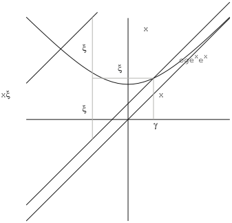
Proof. As seen in Figure 1, when x > γ, the log-sum-exp function log(ex + e-x ) is upper bounded by the linear function x + b, where b is defined as above. On the other hand, as x → -∞, the two functions could deviate at most by 2ξ, where ξ is the distance between x and γ. Hence, the upper bound is x + 2ξ + b. Combining both bounds yields the desired result. The bound works for any γ.
Lemma 3.1 allows us to lower bound the log-likelihood function as follows.
Theorem 3.2.
Proof. We upper bound the partition function as follows:
In order to proceed further, we need to bound ∑V2 e2ξ1+b since ξ1 depends on V2. Let [ · ] = max(0, ·) be the rectification function.
Since [ · ]+ is 1-Lipschitz, and |fj| ≤ 1
We substitute the above result back, and continue the same approximation over all the other Vi to get the desired bound.
Adding an L2 regularization term on w, with a given set of samples of size N, we can train the BM by solving the following optimization problem:
Optimization Problem 3.3.
Here R(w) can be considered as an extra regularization of w, and its weight η0 will be selected according to cross validation. We will justify its importance to generalization performance in Section 4. After training, we predict values of the random variables V by solving:
Optimization Problem 3.4.
In the case of conditional BMs where V = (X, Y), the objective functions above only involve hinge loss terms for variables Y and ignore the loss terms for variables X. The extra penalty term R(w) only contains the weights of those cliques that involve at least two Y vertices. In addition, the partition function of the conditional likelihood does not marginalize over X, and the domain of X can be relaxed to real values. In the rest of this paper, we discuss the conditional BMs for classification tasks, although the algorithms apply to the original BMs as well.
3.1 Relation to other large margin based structural learning methods
Large margin based approaches have been explored extensively in the past few years [Crammer and Singer, 2001; Collins, 2002; Taskar et al., 2004; Tsochantaridis et al., 2004]. The basic idea is that the objective function ∑j wjfj with true assignments of Y must be greater than ones with other assignments by a margin γ. The Structural Support Vector Machine (SSVM) is one approach to this problem that can be solved efficiently [Tsochantaridis et al., 2004; Joachims et al., to appear] by considering only a polynomial number of constraints to achieve optimality. For each added constraint, one has to perform an inference (the "separation oracle"). When exact inference is not available, either performance or correctness is not guaranteed [Finley and Joachims, 2008; Kulesza and Pereira, 2007].
In contrast, the LMBM does not need any inference during training and leads to a fast learning algorithm. Furthermore, we show that the LMBM has a generalization bound with a sample complexity as low as the PAC-Bayes bound of SSVMs.
4 Empirical RiskMinimization and Generalization Bound
The training of SSVMs minimizes the prediction errors empirically, which is considered an advantage over maximum likelihood estimation. Similarly, the objective function of the LMBM also upper bounds the 0-1 error as shown in Theorem 4.1 below. Therefore, the performance of the LMBM can be justified by empirical risk minimization as well.
Theorem 4.1. Consider the decision function defined in O.P 3.4, and let L(x, y,w) = ∑i ξi(x, y,w). If ∀y ̸= ˆy, x, y ∼ D, ∃T > 0, L(x, y, w) > T , then
Proof.
The function 1(z) is the indicator function that is 1 when z is true and 0 for false. H(z) is the Heaviside function that is 1 for z ≥ 0 and 0 otherwise. The last inequality comes from the fact that H(v -T) ≤ vT .
In above theorem, the threshold T is a crucial factor when the expected loss ED[L(x, y,w)] is greater than 0 due to the existence of noise. The larger the T , the better the generalization performance. The threshold T for the LMBM is given below:
Remark 4.2. Let Si = {j|∃k ̸= i, Yi, Yk ∈ Cj}, gj = supx,y |fj(x, y)|, we have T = mini[γ - ∑j∈Si |wj | gj]+
Proof. Let fj = fj(x, y), ˆ fj = fj(x, ˆ y). For any yi ̸= ˆ yi, we have ξi = [γ - A0 - A1]+,ˆ ξi = [γ - A0 - A2]+ where A0 = ∑j:Yi∈Cj∧fj= ˆ fj wjfj,A1 = ∑j:Yi∈Cj∧fj̸= ˆ fj wjfj,A2 = ∑j:Yi∈Cj∧fj̸= ˆ fj wj ˆ fj. Since x is the same, and only y ∈ {-1, 1}K changed, it is easy to verify fj = - ˆ fj, if fj ̸= ˆ fj. So ˆ ξi = [γ -A0 +A1]+. If A1 < 0, we have L > ξi > [γ - A0]+. Otherwise, L > ˆL > ˆ ξi > [γ -A0]+. So L > [γ - ∑j:Yi∈Cj∧fj= ˆ fj wjfj ]+. To make the threshold independent of x, y, we further loosen it to L >mini[γ - ∑j∈Si |wj| gj]+.
If the weights of those cliques that involve at least two Y variables are too large, the threshold is possibly very small, and generalization performance will not be guaranteed. In fact, the extra regularization term R(w) in O.P. 3.3 can keep those weights small to ensure a large threshold. In the experiments, we show that the LMBM with this extra regularization consistently outperforms the one without it. Furthermore, although R(w) contains a L1 term, for the algorithmic simplicity, we replace it with a L2 term.
The convergence rate of a stochastic objective function similar to LMBM's has been studied by Shalev-Shwartz et al. [Shalev-Shwartz et al., 2008], where only one output variable is considered. With Lemma 4.3, Corollary 4 in [ShalevShwartz et al., 2008] can be applied to the objective function of LMBM.
Lemma 4.3. Let F = {x, y ↦→ L(x, y, w)}, Fi = {x, y ↦→ ∑j:Vi∈Cj wjfj(x, y)}, φ(z) = [γ - z]+. We have
Proof.
Here RN is the Rademacher complexity [Bartlett and Mendelson, 2002] of sample size N. See [Bartlett and Mendelson, 2002] for details on the notation.
We can now derive a generalization bound as in Theorem 4.4 below by first defining:
Theorem 4.4. Assuming ∑j ‖fj‖22 < B2 , d is the maximum clique size, for any δ > 0, with probability 1 - δ over the sample size N, if λ = c B√d/δ ‖wo‖√N , where c is a constant,we have
This generalization bound is better than the PAC-Bayes bound for SSVMs by √logN. When the exact inference is intractable, the generalization bound for SSVMs is further worsened due to the extra degrees of freedom introduced by relaxation [Kulesza and Pereira, 2007].
5 Dual Coordinate Descent Method for Large Margin Boltzmann Machines
In this section, we propose a dual coordinate descent method for large margin BMs that shares similarities with the dual coordinate method used for linear SVMs [Hsieh et al., 2008]. The method contains a fast update for each iteration, with a relatively small number of iterations. Unlike nonlinear SVMs, one does not need to re-compute the whole gradient in each iteration, which saves a factor of O(N) time where N is the number of samples.
Consider the optimization problem
where U = 1/(λN) and η are the penalty constants set by cross-validation. If the j th clique contains only one Y variable, ηj = 1, otherwise ηj = η0. Let αil and βil be Lagrange multipliers. Then, we have the Lagrangian:
We optimize L with respect to w and ξ:
Substituting for w and ξ, we have the dual Lagrangian:
The dual coordinate descent algorithm picks αil one at a time and optimizes the dual Lagrangian with respect to this variable:
subject to 0 ≤ αil + d ≤ U
where Qjll = fjl fjl η2 j , ∇ilLα = ∑j:Vi∈Cj wjfjl - γ. The objective has the almost the same form as linear SVMs. The Q matrix satisfies all properties required for convergence described in [Hsieh et al., 2008].
6 Experimental Results
We applied LMBMs to the challenging problem of multilabel classification. We choose four popular benchmark datasets: Scene [Boutell et al., 2004], Yeast [Elisseeff and Weston, 2002], and Mediamill10/Mediamill50 [Snoek et al., 2006]. Mediamill10 selects the first 10 labels and data containing at least one of them. Mediamill50 selects the first 50 labels. The basic characteristics of these datasets are listed in Table 1.
Algorithm 1 The dual coordinate descent algorithm for large margin Boltzmann machines
1: α ← 0, w ← 0 2: while α is not optimal do 3: for all αil do 4: αo ←αil 5: G = ∑j:Vi∈Cj wjfjl -γ 6: PG = { min(G, 0) αo = 0, max(G, 0) αo = U, G 0 < αo < U 7: if |PG| ̸= 0 then 8: αil ← min(max(αo - G Pj:Vi∈Cj Qjll , 0), U) 9: wj ←wj + (αil -αo)fjl, if Vi ∈ Cj 10: end if 11: end for 12: end while 13: returnw| name | train | test | features | labels | weights |
|---|---|---|---|---|---|
| scene | 1211 | 1196 | 294 | 6 | 1788 |
| yeast | 1500 | 917 | 103 | 14 | 1547 |
| mediamill10 | 2718 | 1087 | 120 | 10 | 1255 |
| mediamill50 | 25737 | 10919 | 120 | 50 | 7500 |
LMBM and SSVMmodel the same distribution family, i.e., a completely connected graph with a maximal clique size of two. The approximation algorithm for SSVM implements relaxed linear programming (LP) and is guaranteed to reach a possibly sub-optimal solution in polynomial time [Finley and Joachims, 2008]. In our experiments involving SSVM, we adopt a popular LP relaxation that enforces a marginalization constraint [Wainwright et al., 2005a] and solve it with the software package lp solve. We optimize the margin-rescaling objective with the Hamming loss. For LMBMs, we implement a mixed integer programming (MIP) algorithm for testing and cross-validation. We observe that for the optimization problem 3.4, MIP always outperforms LP, but interestingly, for SSVMs, integer programming produces the same results as LP on these datasets.
Five methods are compared in these experiments: LMBM trained without the extra regularization η0 = 0, LMBMr trained with the extra regularization η0 ̸= 0, SSVM the structural SVM, ILSVM the independent linear SVM that treats Y mutually independent, and MLSVM which transforms the multi-label classification problem into a multi-class classification problem by treating each label combination as one class. According to [Tsoumakas andKatakis, 2007], inYeast and Scene, MLSVM outperforms many other methods, but it is not scalable to large numbers of Y since the number of classes increases exponentially.
In multi-label datasets, the labels are typically highly unbalanced, with negative labels usually outnumbering positive labels. So the Hamming loss (H) is not an informative performance metric. We adopt four additional popular performance metrics: accuracy (A), precision (P), recall (R) and F1 score (F) as defined in Eqn. 3 below, where ˆY are the predicted positive labels and Y are the true positive labels.
For ILSVM, LMBM, LMBMr and SSVM, 5-fold crossvalidation was used to select the parameters individually. For SSVM, C was selected from {0.01, 0.1, 1, 10, 100}. For LMBMr, LMBM and ILSVM, U was selected from {0.01, 0.1, 1, 10, 100}. For LMBMr, η0 was selected from {5, 10, 100}.
The results of MLSVM come from [Tsoumakas and Katakis, 2007]. The metric used in cross-validation is the accuracy (A). We also recorded the training time for each machine trained with the selected optimal parameters. The CPU time is measured on a 2.8Ghz Pentium4 desktop computer.
The final results are shown in Table 2 (↓ means smaller numbers are better while ↑ means the opposite).
A key observation from Table 2 is that LMBMs are consistently orders of magnitude faster than SSVMs and the other algorithms, while producing results that are in the same range as the other methods. The speed of SSVMs depends on the speed of the lp solve and the number of times lp solve is called. The actual number of variables in the relaxed LP is quadratic of the number of labels in the problem. Typically, lp solve solves a 10-variable problem in about 0.01s, and a 50-variable problem in about 2s. In our experiments, SSVMs fails to produce results for Mediamill50 in 10 hours. For smaller scale problems such as Scene and Yeast, MLSVM can outperform LMBMr but MLSVM becomes exponentially expensive as the number of labels increases, and the sample complexity increases exponentially as well. ILSVM performs well on Mediamill10 and Mediamill50 since the labels are relatively independent of each other, but the performance drops when there are dependencies among labels as in Scene. Both LMBM and SSVM perform well in datasets with strong label-dependency, but not in datasets with weak labeldependency. LMBMr demonstrates good performance on both types of datasets, which might indicate that the threshold T is the key factor governing generalization performance.
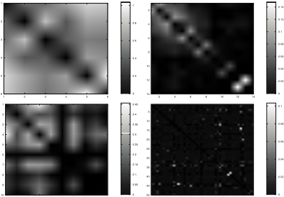
More importantly, LMBMr is able to model the dependency structure among the variables that leads to improved accuracy (A) of prediction compared with ILSVM. Figure 2 shows the different dependency patterns discovered by LMBMr for the different datasets. Interestingly, the dependency pattern changes significantly from small scale problems to large scale problems. For example, in Mediamill10, the label 4 (outdoor) has a strong correlation (negative) with the label 1 (people) and a weak correlation (positive) with label 10 (crowd). But in Mediamill50, the correlation between people and outdoor disappears, while the weak correlation between crowd and outdoor remains. Another interesting characteristic of the Mediamill50 dataset is that unlike the other three datasets, the most frequent labels (upper left portion of the weights matrix) appear relatively independent of each other, while the least frequent labels (lower right portion of the weights matrix) tend to have stronger correlations with the others.
| Scene | ||||||
|---|---|---|---|---|---|---|
| Method | time(s)↓ | H↓ | A↑ | P↑ | R↑ | F↑ |
| ILSVM | 0.63 | 0.109 | 0.567 | 0.782 | 0.605 | 0.682 |
| LMBM | 0.25 | 0.108 | 0.681 | 0.721 | 0.686 | 0.703 |
| LMBMr | 0.24 | 0.107 | 0.682 | 0.722 | 0.687 | 0.704 |
| SSVM | 81.8 | 0.100 | 0.619 | 0.795 | 0.635 | 0.706 |
| MLSVM | N.A. | 0.100 | 0.704 | 0.713 | 0.737 | 0.725 |
| Yeast | ||||||
| Method | time(s)↓ | H↓ | A↑ | P↑ | R↑ | F↑ |
| ILSVM | 0.95 | 0.199 | 0.498 | 0.717 | 0.570 | 0.635 |
| LMBM | 0.47 | 0.368 | 0.329 | 0.414 | 0.561 | 0.476 |
| LMBMr | 0.36 | 0.199 | 0.504 | 0.709 | 0.584 | 0.640 |
| SSVM | 81.7 | 0.233 | 0.337 | 0.748 | 0.337 | 0.465 |
| MLSVM | N.A. | 0.206 | 0.530 | 0.615 | 0.672 | 0.642 |
| Mediamill10 | ||||||
| Method | time(s)↓ | H↓ | A↑ | P↑ | R↑ | F↑ |
| ILSVM | 75.57 | 0.049 | 0.636 | 0.859 | 0.636 | 0.731 |
| LMBM | 36.36 | 0.082 | 0.603 | 0.605 | 0.603 | 0.604 |
| LMBMr | 45.2 | 0.052 | 0.731 | 0.752 | 0.731 | 0.741 |
| SSVM | 459.9 | 0.082 | 0.589 | 0.609 | 0.589 | 0.599 |
| Mediamill50 | ||||||
| Method | time(s)↓ | H↓ | A↑ | P↑ | R↑ | F↑ |
| ILSVM | 32.29 | 0.025 | 0.480 | 0.739 | 0.480 | 0.582 |
| LMBM | 49.53 | 0.225 | 0.044 | 0.048 | 0.286 | 0.082 |
| LMBMr | 33.00 | 0.025 | 0.480 | 0.741 | 0.480 | 0.583 |
| SSVM | > 10hrs | |||||
7 Conclusions and Future work
We have proposed an efficient SVM-style learning algorithm for Boltzmann machines based on a new large-margin variational approximation to the partition function. For multi-label classification tasks, these large margin Boltzmann machines provide an efficient alternative to recently proposed structural SVMs. Experimental results on four benchmark multi-label classification problems demonstrate that LMBMs are significantly faster than existing approaches and can match or beat the performance of other methods.
Several challenges and open questions remain. For example, can a better approximation be achieved through the use of hidden variables in large margin Boltzmann machines? Although the learning algorithm for LMBMs is fast, the inference is still slow and approximate. To address this problem, we have recently explored large margin directed Boltzmann machines (LMDBMs) that can again be trained using an SVM-style objective function [Miao and Rao, 2009]. More importantly, for LMDBMs, there exists a branch and bound exact inference algorithm that is many orders of magnitude faster than LP.
1
2
3
4
5
6
7
8
9
10
5
10
15
20
25
30
35
40
45
50
Figure 2: The different dependency structures discovered by LMBMr for different datasets. The colorbar of each figure shows the scale of weights in terms of the gray level(absolute value). The top row, left to right: Scene and Yeast; The bottom row, left to right: Mediamill10 andMediamill50.
Acknowledgments
We would like to thank Andrew Guillory, James Lee, Aaron Shon, and the anonymous reviewers for valuable suggestions.
@inproceedings{ijcai2009p195,
  title     = {Large Margin Boltzmann Machines},
  author    = {Miao, Xu and Rao, Rajesh P. N.},
  booktitle = {Proceedings of the Twenty-First International Joint Conference on
               Artificial Intelligence, {IJCAI-09}},
  publisher = {International Joint Conferences on Artificial Intelligence},
  editor    = {Craig Boutilier},
  pages     = {1156--1161},
  year      = {2009},
  url       = {https://ijcai.org/proceedings/2009/195},
}
TY - CPAPER TI - Large Margin Boltzmann Machines AU - Miao, Xu AU - Rao, Rajesh P. N. T2 - Proceedings of the Twenty-First International Joint Conference on Artificial Intelligence, IJCAI-09 PB - International Joint Conferences on Artificial Intelligence PY - 2009 SP - 1156 EP - 1161 UR - https://ijcai.org/proceedings/2009/195 ER -Copied
Machine-readable versions of this paper, for tools and AI agents:





