
FRACTAL: Efficient Fault Isolation Using Active Testing
Proceedings of the Twenty-First International Joint Conference on Artificial Intelligence. Pages 778-783.
© 2009 International Joint Conferences on Artificial Intelligence
Abstract
Model-Based Diagnosis (MBD) approaches often yield a large number of diagnoses, severely limiting their practical utility. This paper presents a novel active testing approach based on MBD techniques, called FRACTAL (FRamework for ACtive Testing ALgorithms), which, given a system description, computes a sequence of control settings for reducing the number of diagnoses. The approach complements probing, sequential diagnosis, and ATPG, and applies to systems where additional tests are restricted to setting a subset of the existing system inputs while observing the existing outputs. This paper evaluates the optimality of FRACTAL, both theoretically and empirically. FRACTAL generates test vectors using a greedy, next-best strategy and a low-cost approximation of diagnostic information entropy. Further, the approximate sequence computed by FRACTAL's greedy approach is optimal over all poly-time approximation algorithms, a fact which we confirm empirically. Extensive experimentation with ISCAS85 combinational circuits shows that FRACTAL reduces the number of remaining diagnoses according to a steep geometric decay function, even when only a fraction of inputs are available for active testing.Alexander Feldman, Gregory Provan, Arjan van Gemund
- [Alur et al., 1995] Rajeev Alur, Costas Courcoubetis, and Mihalis Yannakakis. Distinguishing tests for nondetermin- istic and probabilistic machines. In Proc. ACM Symposium on Theory of Computing, pages 363-372, 1995.
- [Andreas Krause et al., 2008] A. Andreas Krause, H. Bren- dan McMahan, Carlos Guestrin, and Anupam Gupta. Ro- bust submodular observation selection. Journal of Ma- chine Learning Research, 9:2761-2801, 2008.
- [Brglez and Fujiwara, 1985] Franc Brglez and Hideo Fuji- wara. A neutral netlist of 10 combinational benchmark cir- cuits and a target translator in Fortran. In Proc. ISCAS'85, pages 695-698, 1985.
- [Brodie et al., 2003] Mark Brodie, Irina Rish, Sheng Ma, and Natalia Odintsova. Active probing strategies for prob- lem diagnosis in distributed systems. In Proc. IJCAI'03, pages 1337-1338, 2003.
- [de Kleer and Williams, 1987] Johan de Kleer and Brian Williams. Diagnosing multiple faults. Artificial Intelli- gence, 32(1):97-130, 1987.
- [Esser and Struss, 2007] Michael Esser and Peter Struss. Fault-model-based test generation for embedded software. In Proc. IJCAI'07, 2007. IJCAI
- [Feige, 1998] Uriel Feige. A threshold of ln n for approxi- mating set cover. Journal of ACM, 45(4):634-652, 1998.
- [Heinz and Sachenbacher, 2008] Stefan Heinz and Martin Sachenbacher. Using model counting to find optimal dis- tinguishing tests. In Proc. of COUNTING'08, pages 91- 106, 2008.
- [Krause and Guestrin, 2007] Andreas Krause and Carlos Guestrin. Near-optimal observation selection using sub- modular functions. In Proc. AAAI'07, pages 1650-1654, 2007.
- [Kuhn et al., 2008] Lukas Kuhn, Bob Price, Johan de Kleer, Minh Do, and Rong Zhou. Pervasive diagnosis: Integra- tion of active diagnosis into production plans. In Proc. DX'08, pages 106-119, 2008.
- [Kundakcioglu and Ünlüyurt, 2007] O. Erhun Kundakcioglu and Tonguc ¸Ünlüyurt. Bottom-up construction of mini- mum-cost and/or trees for sequential fault diagnosis. IEEE Trans. on SMC, 37(5):621-629, 2007.
- [McCormick, 2005] S. Thomas McCormick. Handbooks in Operations Research and Management Science, vol- ume 12, chapter Submodular Function Minimization, pages 321-391. Elsevier, 2005.
- [Nemhauser et al., 1978] George Nemhauser, Laurence Wolsey, and Marshall Fisher. An analysis of approxi- mations for maximizing submodular set functions -I. Mathematical Programming, 14(1):165-294, 1978.
- [Pattipati and Alexandridis, 1990] Krishna Pattipati and Mark Alexandridis. Application of heuristic search and information theory to sequential fault diagnosis. IEEE Trans. on SMC, 20(4):872-887, 1990.
- [Raghavan et al., 1999] Vijaya Raghavan, Mojdeh Shakeri, and Krishna Pattipati. Optimal and near-optimal test se- quencing algorithms with realistic test models. IEEE Trans. on SMC, 29(1):11-26, 1999.
- [Siddiqi and Huang, 2007] Sajjad Siddiqi and Jinbo Huang. Hierarchical diagnosis of multiple faults. In Proc. IJ- CAI'07, pages 581-586, 2007. IJCAI
- [Stephan et al., 1996] Paul Stephan, Robert Brayton, and Al- berto Sangiovanni-Vincentelli. Combinational test genera- tion using satisfiability. IEEE Trans. on CAD of Integrated Circuits and Systems, 15(9):1167-1176, 1996.
- [Struss, 1994] Peter Struss. Testing physical systems. In Proc. AAAI'94, pages 251-256, 1994.
- [Tu and Pattipati, 2003] Fang Tu and Krishna Pattipati. Roll- out strategies for sequential fault diagnosis. IEEE Trans. on SMC, 33(1):86-99, 2003.
References were extracted automatically from the PDF and may contain errors.
Full text extracted automatically from the PDF; figures, tables and equations may differ. The PDF is the version of record.
1 Introduction
The number of diagnoses generated by a Model-Based Diagnosis (MBD) engine (e.g., the General Diagnostic Engine [de Kleer and Williams, 1987]) can be large, and in the worstcase is exponential in the number of components. This ambiguity (uncertainty) of the diagnostic result arises due to to modeling uncertainty (e.g., modeling weakness due to ignorance of abnormal behavior or the need for robustness) and the limited number of observations (sensor-lean systems, limited observation horizons) of typical systems, especially when false positives cannot be tolerated.
Given a set of plausible diagnoses, in certain situations one can devise additional tests (probes), that reduce the diagnostic ambiguity [de Kleer and Williams, 1987]. Because most systems are sensor-lean, there is a limited set of test points that can be used to further narrow down the diagnostic solution space. Many systems have built-in testing capabilities with pre-defined test vectors; the drawback with such pre-specified test strategies is that they must cover all possible faults and observations, and so are typically highly sub-optimal.
Rather than rely on predefined test-vectors, either computed to expose particular faults (ATPG, e.g., [Stephan et al., 1996]), or selected from a limited test matrix (sequential diagnosis, e.g., [Pattipati and Alexandridis, 1990]), we propose a novel, active testing strategy, which dynamically determines test vectors from the entire test vector space using an MBD approach. An active testing problem takes as input a system model, an initial observation and a diagnosis, and computes the set of input test vectors that will minimize diagnostic ambiguity with the least number of test vectors. The test vectors are computed by setting a subset of input settings which, together with the resulting output values, optimally reduce the size of the set of diagnoses. To the best of our knowledge, our definition of and solution for active testing are novel. Furthermore, our method is based on MBD, which requires few assumptions about the model and the observations.
Our contributions are as follows. (1) We define the active testing problem and outline a strategy, FRACTAL, which generates test vectors using a greedy, next-best policy and a low-cost approximation of diagnostic information entropy to guide the search. (2) We empirically demonstrate that FRACTAL computes an expected number of diagnoses which shows near 87% correlation with the exact number of remaining diagnoses. (3) We prove that FRACTAL's greedy approach computes an approximate solution which is optimal over all approximation algorithms, a fact which we confirm empirically. (4) We present extensive empirical data on ISCAS85 circuits, which shows that FRACTAL reduces the number of remaining diagnoses according to a geometric decay function (e.g., reducing 46003 double faults in c7552 to 4 in 6 steps only), even when only a fraction of the inputs are modifiable.
2 RelatedWork
Early work aimed at diagnostic convergence is the approach by de Kleer and Williams [1987] which computes the probe sequence that reduces diagnostic entropy using a myopic search strategy. Unlike their work, in active testing we assume that probes are not available, other than indirectly exposed through diagnosis based on test vectors, which offers an automated solution.
Generating test vectors to deduce faults has received considerable attention. Automatic test pattern generation (ATPG) aims at verifying particular, single-faults [Stephan et al., 1996]. ATPG differs from active testing in that the vectors are specific for particular single-faults, whereas active testing generates a sequence of vectors to isolate unknown, multiplefaults, a much harder problem.
Active testing bears some resemblance with sequential diagnosis, which also generates a sequence of test vectors [Pattipati and Alexandridis, 1990; Raghavan et al., 1999; Tu and Pattipati, 2003; Kundakcioglu and ¨Unl¨uyurt, 2007]. The principle difference is that in sequential diagnosis a fault dictionary is used ("fault matrix"). This pre-compiled dictionary has the following drawback: in order to limit the (exponential) size of the dictionary, the number of stored test vectors is extremely small compared to the test vector space. This severely constrains the optimality of the vector sequence that can be generated, compared to active testing, where test vectors are computed on the fly using a model-based approach. Furthermore, the matrix specifies tests that only have a binary (pass/fail) outcome, whereas active testing exploits all the system's outputs, leading to faster diagnostic convergence. In addition, we allow the inputs to be dynamic, which makes our framework suitable for online fault isolation.
Model-Based Testing (MBT) [Struss, 1994] is a generalization of sequential diagnosis. The purpose of MBT is to compute inputs manifesting a certain (faulty) behavior. The main differences from our active testing approach are that MBT (1) assumes that all inputs are controllable and (2) MBT aims at confirming single faulty behavior as opposed to maximally decreasing the diagnostic uncertainty.
Our task is harder than that of Raghavan et al. [1999], since despite the diagnosis lookup using a fault dictionary, the diagnosis task is NP-hard; in our case we compute a new diagnosis after every test. Hence we have an NP-hard sequential problem interleaved with the complexity of diagnostic inference at each step (in our case the complexity of diagnosis is Σp2 -hard). Apart from the above-mentioned differences, we note that optimal test sequencing is infeasible for the size of problems in which we are interested.
A recent approach to active diagnosis is described by Kuhn et al. [2008], where additional test vectors are computed to optimize the diagnosis while the system (a copier) remains operational. Their work differs from ours in that plans (roughly analogous to test sequences) with a probability of failure T are computed statically, and a plan remains unmodified even if it fails to achieve its desired goal (a manifestation of a failure with probability close to T). Conversely, FRACTAL dynamically computes next-best control settings in a game-like manner.
Rish et al. [2003] cast their models in terms of Bayesian networks. Our notion of entropy is the size of the diagnosis space, whereas Rish et al. use decision-theoretic notions of entropy to guide test selection.
Our use of greedy algorithms over a submodular function is analogous to the observation-selection problem of [Krause and Guestrin, 2007; Andreas Krause et al., 2008] used for design of sensor-networks and experiments. Whereas Krause et al. use the submodularity of variance-minimization or information-gain of sensor readings, we use the submodularity of diagnosis-updating given new tests.
We solve a different problem than that of Heinz and Sachenbacher [2008] or Alur et al. [1995]. Our framework assumes a static system (plant model) for which we must compute a temporal sequence of tests to best isolate the diagnosis. In contrast, Heinz and Sachenbacher [2008] and Alur et al. [1995] assume a non-deterministic system defined as an automaton. Esser and Struss [2007] also adopt an automaton framework for test generation, except that, unlike Heinz and Sachenbacher [2008] or Alur et al. [1995], they transform this automation to a relational specification, and apply their framework to software diagnosis. This automaton-based framework accommodates more general situations than does ours, such as the possibility that the system's state after a transition may not be uniquely determined by the state before the transition and the input, and/or the system's state may be associated with several possible observations. In our MBD framework, a test consists of an instantiation of several variables, which corresponds to the notion of test sequence within the automaton framework of Heinz and Sachenbacher [2008].
3 Active Testing
Our discussion starts by adopting relevant MBD notions.
3.1 Concepts and Definitions
A model of a system is a propositional Wff.
Definition 1 (Active Testing System). An active testing system ATS is defined as ATS = 〈SD, COMPS, CTL, OBS〉, where SD is a propositional Wff over a variables set V , COMPS∪OBS∪CTL ⊆ V , and COMPS, OBS, and CTL are sets containing assumable, observable, and control variables, respectively.
Throughout this paper we assume that OBS, COMPS, and CTL are disjoint, and SD ̸|=⊥. Sometimes it is convenient (but not necessary) to split OBS into non-controllable inputs IN and outputs OUT (OBS = IN ∪ OUT, IN ∩ OUT = ∅).
Definition 2 (Diagnosis). Given a system ATS, an observation α over some variables in OBS, and an assignment ω to all variables in COMPS, ω is a diagnosis iff SD∧α∧ω ̸|=⊥.
The set of all diagnoses of SD and an observation α is denoted as Ω(SD, α). The cardinality of a diagnosis, denoted as |ω|, is defined as the number of negative literals in ω.
Definition 3 (Minimal-Cardinality Diagnosis). A diagnosis ω≤ is defined as Minimal-Cardinality (MC) if no diagnosis ˜ω≤ exists such that |˜ω≤| < |ω≤|.
Our selection of minimality criterion is such that it is impossible to compute all diagnoses from the set of all MC diagnoses without further inference. MC diagnoses, however, are often used in practice due to the prohibitive cost of computing a representation of all diagnoses of a system and an observation (e.g., all subset-minimal diagnoses).
The number of MC diagnoses of a system ATS and an observation α is denoted as |Ω≤(SD, α)|, where Ω≤(SD, α) is the set of all MC diagnoses of SD ∧ α. Given a system ATS, an observation sequence S is defined as a k-tuple of terms S = 〈α1, α2, . . . , αk〉, where αi (1 ≤ i ≤ k) is an instantiation of variables in OBS.
Throughout this paper, we assume that the health of the system under test does not change during the test (i.e., the same inputs and a fault produce the same outputs) and call this assumption stationary health.
Lemma 1. Given a system ATS, a health state for its components ω, and an observation sequence S, it follows that ω ∈ Ω(SD, α1) ∩ Ω(SD, α2) ∩ . . . ∩ Ω(SD, αk).
Proof. The above statement follows immediately from the stationary health assumption and Def. 2.
Lemma 1 can be applied only in the cases in which all diagnoses are considered. If we compute subset-minimal diagnoses in a weak-fault model, for example, the intersection operator has to be redefined to handle subsumptions. To handle non-characterizing sets of diagnoses (e.g., MC or first m diagnoses), we provide the following definition.
Definition 4 (Consistency-Based Intersection). Given a set of diagnoses D of SD ∧ α, and a posteriori observation α′ , the intersection of D with the diagnoses of SD ∧ α′ , denoted as Ω∩(D, α′ ), is defined as the set D′ (D′ ⊆ D) such that for each ω ∈ D′ it holds that SD ∧ α′ ∧ ω ̸|=⊥.
It is straightforward to generalize the above definition to an observation sequence S.
Definition 5 (Remaining Minimal-Cardinality Diagnoses). Given a diagnostic system ATS and an observation sequence S, the set of remaining diagnoses Ω(S) is defined as Ω(S) = Ω∩(Ω∩(· · · Ω∩(Ω≤(SD, α1), α2), · · · ), αk).
We use |Ω(S)| instead of the more precise diagnostic entropy as defined by de Kleer et al. [de Kleer and Williams, 1987] and subsequent works, as this allows low-complexity estimations (discussed in Sec. 3.3). In particular, if all diagnoses are of minimal-cardinality and the failure probability of each component is the same, then the gain in the diagnostic entropy can be directly computed from |Ω(S)|.
3.2 Control Strategy
We assume that we have an underlying set S = 〈S1, . . . , Sq〉 of possible observations, where each observation Si ∈ S consists of Si = αi ∧ γi, for whiche we are given as (non-modifiable) inputs the sequence of OBS assignments 〈α1, α2, . . . , αk〉, and we must choose a sequence Γ = 〈γ1, γ2, . . . , γl〉, l ≤ k - 1 of controls to minimize the set of remaining diagnoses. We set f(γ) = |Ω(S)| for some S ⊆ S. Our AT problem is defined as follows:
Problem 1 (Optimal Control Input). Given a system ATS, and a sequence S = 〈α1 ∧ γ1, α2, . . . , αk〉, where αi (1 ≤ i ≤ k) are OBS assignments and γ1 is a CTL assignment, compute a sequence of CTL assignments γ ∗ = γ2, . . . , γk, such that γ ∗ = minγ⊆Γ f (γ).
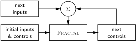
Although our framework also allows us to skip the requirements of an initial observation, 1 in practice, active testing is triggered by a failure, hence the initial observation. While similar to classic, sequential diagnosis, this is different from ATPG as we don't compute tests for a specific target diagnosis ω∗ (in which case there is no need to have an initial control γ and observation α). In the active testing problem, the situation is different: we target any health state, so an initial observation and control are required. The computational architecture in which we use FRACTAL is illustrated by Fig. 1.
1 In our presentation "sequential diagnosis" is used in the MBD context, which is slightly different from its original presentation, but still compatible.
In practice, a diagnostician does not know what the next observation will be. Fully solving an active testing problem would necessitate the conceptual generation of a tree with all possible observations and associated control assignments in order to choose the sequence that, on average, constitutes the shortest (optimal) path over all possible assignments.
The sequential diagnosis problem studies optimal trees when there is a cost associated with each test [Tu and Pattipati, 2003]. When costs are equal, it can be shown that the optimization problem reduces to a next best control problem (assuming one uses information entropy). In this paper a diagnostician who is given a sequence S and who tries to compute the next optimal control assignment would try to minimize the expected number of remaining diagnoses |Ω(S)|.
3.3 Expected Intersection Size
We will compute the expected number of diagnoses for a set of observable variables M (M ⊆ OBS). The initial observation α and the set of MC diagnoses D = Ω≤(SD, α) modify the probability density function (pdf) of subsequent outputs (observations), i.e., a subsequent observation α′ changes its likelihood. The (non-normalized) a posteriori probability of an observation α′ , given an MC operator and an initial observation α is:
The above formula comes by quantifying how a given a priori set of diagnoses restricts the possible outputs (i.e., we take as probability the ratio of the number of remaining diagnoses to the number of initial diagnoses). In practice, there are many α for which Pr(α′ |SD, α) = 0, because a certain fault heavily restricts the possible outputs of a system (i.e., the set of the remaining diagnoses in the nominator is empty).
The expected number of remaining MC diagnoses for a variable set M, given an initial observation α, is then the weighted average of the intersection sizes of all possible instantiations over the variables in M (the weight is the probability of an output):
where D = Ω≤(SD, α) and M ∗ is the set of all possible assignment to the variables in M. Replacing (1) in (2) and simplifying gives us the following definition:
Definition 6 (Expected Minimal-Cardinality Diagnoses Intersection Size). Given a system ATS and an initial observation α, the expected remaining number of MC diagnoses E≤(SD,OBS|α) is defined as:
where OBS∗ is the set of all possible assignments to all variables in OBS.
4 An Algorithm for Active Testing
As the active testing problem is extremely complex (counting the number of MC diagnoses, computing the expectation for the number of MC diagnoses and finding the optimal control setting are all NP-hard or worse problems), we propose a stochastic approach.
4.1 Approximation of the Expectation
Our algorithm for active testing consists of (1) a randomized algorithm for approximating the expected number of remaining diagnoses and (2) a greedy algorithm for searching the space of control assignments. We continue our discussion with approximating the expectation.
The key insight which allows us to build a faster method for computing the expected number of remaining diagnoses is that the prior observation (and respectively the set of MC diagnoses) shifts the probability of the outputs. Hence, an algorithm which samples the possible input assignments (it is safe to assume that inputs are equally likely) and counts the number of different observations, given the set of prior diagnoses, would produce a good approximation.
Algorithm 1 uses a couple of auxiliary functions: RANDOMINPUTS assigns random values to all inputs and INFEROUTPUTS computes all outputs from the system model, all inputs and a diagnosis. 2 The computation of the intersection size |Ω∩(D, α∧β∧γ)| can be implemented by counting those ω ∈ D for which SD ∧ α ∧ β ∧ γ ∧ ω ̸|=⊥.
The algorithm terminates when a termination criterion (checked by TERMINATE) is satisfied. In our implementation TERMINATE returns success when the last n iterations (where n is a small constant) leave the expected number of diagnoses, ˆE, unchanged. Our experiments show that for all problems considered, n < 100 yields a negligible error.
4.2 Greedy Control Algorithm
Algorithm 2 computes a control assignment for a given active testing system and a prior observation by assuming that the control literals are independent, flipping them one at a time, and accepting a new control assignment if it decreases ˆE.
The set of initial diagnoses is computed from the initial observation in line 2. In line 5, Alg. 2 "flips" the next literal in the
2 This is not always possible in the general case. In our framework, we have a number of assumptions, i.e., a weak-fault model, well-formed circuit, etc. The complexity of INFEROUTPUTS varies on the framework and the assumptions.
Algorithm 1 Approximate expectation
1: function EXPECTATION(ATS, γ,D) returns a real inputs: ATS, active testing system γ, term, system configuration D, set of diagnoses, prior diagnoses local variables: α, β, ω, terms s, q, integers, initially 0 Z, set of terms, samples, initially ∅ ˆE, real, expectation 2: repeat 3: α ← RANDOMINPUTS(SD, IN) 4: for all ω ∈ D do 5: β ← INFEROUTPUTS(SD, OUT, α ∧ γ, ω) 6: if α ∧ β ̸∈ Z then 7: Z ← Z ∪ {α ∧ β} 8: s ← s + |Ω∩(D, α ∧ β ∧ γ)| 9: q ← q + |Ω∩(D, α ∧ β ∧ γ)|2 10: ˆE ← q/s 11: end if 12: end for 13: until TERMINATE( ˆE) 14: return ˆE 15: end functioncurrent control assignment. The auxiliary FLIPLITERAL subroutine simply changes the sign of a specified literal in a term. After each "flip" the expected intersection size is computed with a call to EXPECTATION (cf. Alg. 1). If the new expected intersection size is smaller than the current one, then the proposed control assignment is accepted as the current control assignment, and the search continues from there.
While the active-testing problem is worst-case NP-hard (it can be reduced to computing a diagnosis), as we will see in the experimentation section, it is possible to achieve very good average-case performance by choosing an appropriate MBD oracle. The advantage of the greedy approach, in particular, is that the number of computations of the expected number of diagnoses is linear in the number of literals in the control assignment. This is done at the price of some optimality (i.e., the effect of combinations of controls is neglected).
4.3 Optimality
We now show how the submodularity of our AT problem (Problem 1) means that our greedy approach is as accurate as any poly-time approximation algorithm. Submodular functions are a key concept in combinatorial optimization [Nemhauser et al., 1978;McCormick, 2005]. Intuitively, submodularity highlights the notion that, as we select more observations during active testing, the value of the remaining unselected observations decreases, i.e., we have diminishing returns for successive tests.
In performing inference on a submodular function, we assume that we have a diagnosis evaluation oracle ζ, such that, when given as input a set S ⊆ S, ζ outputs f(S). As a consequence, our submodular function can be solved using polynomially many queries to the oracle ζ.
We define submodularity as follows [Nemhauser et al., 1978]: Given a set function f (S) defined on subsets S ⊆ S of
Algorithm 2 Best next control input
1: function CONTROL(ATS, α) returns a control term inputs: ATS, active testing system α, term, initial observation local variables: γ, γ ′ , terms, control configurations E,E′ , reals, expectations D, set of terms, diagnoses l, literal, control literal 2: D←Ω≤(SD, α) 3: E ← EXPECTATION(ATS, γ,D) 4: for all l ∈ γ do 5: γ ′ ← FLIPLITERAL(γ, l) 6: E′ ← EXPECTATION(ATS, γ ′ , D) 7: if E′ < E then 8: γ ← γ ′ 9: E ← E′ 10: end if 11: end for 12: return γ 13: end functiona universal set, S is said to be submodular if for any two sets A, B ⊆ S, we have f (A) + f (B) ≥ f (A ∪ B) + f (A ∩ B). For our AT application, we define our set function as f(γ) = |Ω(S)| for some S ⊆ S.
Proof. By the definition of submodularity, for any two CTL observation vectors γ1 and γ2 from Γ, we must show that f(γ1) + f(γ2) ≥ f(γ1 ∪ γ2) + f (γ1 ∩ γ2). We define ζi = γi ∧ αi, so that f(α) = |Ω(α ∧ γ)|.
By the law of set-intersection, and using the definition that Ω(S) = ⋂ζi∈S Ω(ζi), we have |Ω(ζ1)| + |Ω(ζ2)| = |Ω(ζ1) ∪ Ω(ζ2)| + |Ω(ζ1) ∩ Ω(ζ2)|. This gives us f(γ1) + f(γ2) ≤ f (γ1 ∪ γ2) + f (γ1 ∩ γ2), which is our desired submodularity condition.
Next, we employ some well-studied results about the optimality of greedy algorithms on submodular functions. First, it has been shown that a greedy algorithm provides a constantfactor approximation for submodular problems.
Lemma 3 (Nemhauser et al., [1978]). For any normalized, monotonic submodular function f, the set S ∗ obtained by a greedy algorithm achieves at least a constant fraction 1-e-1 of the objective value obtained by the optimal solution, i.e.,
where k is a bound on the number of observation vectors we can address.
Moreover, Feige [1998] has shown that the (1 - 1/e)- approximation obtained for such problems using a greedy algorithm is optimal unless P = NP. Together, these results indicate the following:
Theorem 1. Algorithm 2, which is a greedy algorithm, provides a constant-factor approximation to the optimal test sequence, such that no poly-time algorithm can provide a better approximation unless P = NP.
Proof. Follows from Lemmas 2 and 3, and the result in the paper of Feige [1998].
5 Experimental Results
We have experimented on the well-known benchmark models of ISCAS85 circuits [Brglez and Fujiwara, 1985]. In order to use the same model for both MC diagnosis counting and simulation, the fault mode of each logic gate is "stuckat-opposite", i.e., when faulty, the output of a gate assumes the opposite value from the nominal. In addition to the original ISCAS85 models, we have performed cone reductions as described by Siddiqi et al. [Siddiqi and Huang, 2007].
5.1 Experimental Setup
To illustrate the significant diagnostic convergence that is possible, we need initial observations leading to high numbers of initial MC diagnoses. For each circuit, from 1 000 random, non-masking, double-fault observations, we have taken the 100 with the greatest number of MC diagnoses. The mean number of MC diagnoses varies between 166 (in c432) and 23641 (in c7552).
Given inputs, outputs and controls, FRACTAL approximates the optimal control settings. The default control policy of FRACTAL is to apply Alg. 2, a greedy policy. We compare it to (1) a random policy where at each time step we assign an equally-probable random value to each control and (2) to an optimal control policy, where at each time step an exhaustive brute-force search is applied to all control variables.
We define two policies for generating next inputs: random and persistent. The persistent input policy (when the input values do not change in time) is a typical diagnostic worstcase for system environments which are, for example, paused pending diagnostic investigation, and it provides us with useful bounds for analyzing FRACTAL's performance. Combining control and input policies gives us six different experimental setups for our framework.
5.2 Diagnostic Convergence
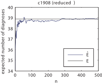
The error of Alg. 1 is not sensitive to the number or the composition of the input variables (extensive experimentation with all circuits showed that for n < 100 we have ˆE within 95% of the true value of E). The value of the expected number of diagnoses ˆE approaches the exact value E when increasing the number of samples. Figure 2 shows an example of ˆE approaching E for c1908.
ISCAS85 has no concept of control variables, hence we "abuse" the benchmark by assigning a fraction of the input variables as controls. It is important to note that turning even a small number of input variables into controls allows for a geometric decay of the diagnostic ambiguity. Figure 3 shows the reduction of the expected number of MC diagnoses as a function of (1) the number of control variables and (2) sequence number. One can observe that a global optimum is reached quickly on both independent axes. Note that Fig. 3 shows an average over 10 pseudo-random experiments for reducing the noise due to the stochastic nature of the algorithm.
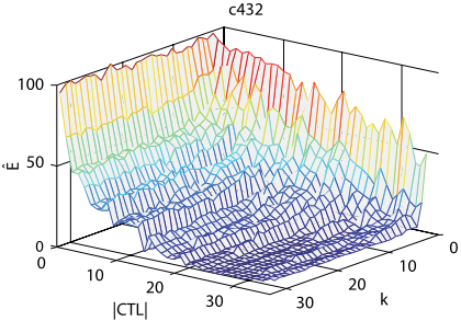
Our results show that ˆ E correlates well with |Ω(S)|. The minimum, maximum, and mean Pearson's linear correlation coefficient for each number of control variables in this example is ρmin = 0.897, ρmax = 0.995, and ρavg = 0.974.
We have repeated the latter experiment with the reduced c880. The results are similar to the non-reduced c880, and the pairwise correlation coefficients are ρmin = 0.68, ρmax = 0.995, and ρavg = 0.94. Hence, identification of cones helps the performance of the diagnostic oracle, but does not degrade convergence behavior.
To summarize the effect of the number of controls on the diagnostic convergence, we fit a geometric decay curve N (k) = N0 · pk + N∞ to Ω(S) for each initial observation and various |CTL|. N0 is the initial number of diagnoses, N∞ is the value to which |Ω(S)| converges, and p is the decay constant. For p = 0.5, N (k) halves every step, like in binary search, hence p corresponds to one bit. For p = 0.25, p corresponds to two bits, etc.
Table 1 shows the average p for various numbers of control bits b = lg |CTL|. The goodness-of-fit criterion R2 for all our experiments is in the range 0.75 - 0.9, except for a small number of cases in which R2 = 1 due to one-step minimization of Ω(S). The table demonstrates that the diagnostic convergence generally improves with |CTL|, but that even with small |CTL| better convergence is achieved than in sequential diagnosis (p = 0.5 on average).
| original | reduced | ||||||
|---|---|---|---|---|---|---|---|
| id | |IN| | 3 bits | 4 bits | 5 bits | 3 bits | 4 bits | 5 bits |
| c432 | 36 | 0.61 | 0.69 | 0.42 | 0.7 | 0.71 | 0.57 |
| c499 | 41 | 0.79 | 0.83 | 0.77 | 0.58 | 0.62 | 0.52 |
| c880 | 60 | 0.5 | 0.55 | 0.62 | 0.49 | 0.47 | 0.44 |
| c1355 | 41 | 0.71 | 0.72 | 0.59 | 0.8 | 0.82 | 0.75 |
| c1908 | 33 | 0.68 | 0.7 | 0.41 | 0.54 | 0.52 | 0.3 |
| c2670 | 233 | 0.45 | 0.49 | 0.39 | 0.39 | 0.44 | 0.42 |
| c3540 | 50 | 0.39 | 0.38 | 0.43 | 0.79 | 0.8 | 0.61 |
| c5315 | 178 | 0.52 | 0.62 | 0.67 | 0.81 | 0.72 | 0.79 |
| c6288 | 32 | 0.31 | 0.41 | 0.23 | 0.64 | 0.7 | 0.59 |
| c7552 | 207 | 0.62 | 0.77 | 0.3 | 0.59 | 0.34 | 0.38 |
Similar to our previous experiments we characterize the convergence of the greedy fractal policy by computing the average p over all observations. This time we have computed p for a fixed CTL, where a quarter of the initial inputs are used as controls. The resulting p, as well as the goodness-offit criterion R2 , for the random and persistent input policies are shown in Table 2.
| original | reduced | |||||||
|---|---|---|---|---|---|---|---|---|
| persistent | random | persistent | random | |||||
| id | p | R2 | p | R2 | p | R2 | p | R2 |
| c432 | 0.7 | 0.85 | 0.62 | 0.93 | 0.64 | 0.88 | 0.76 | 0.9 |
| c499 | 0.81 | 0.89 | 0.78 | 0.89 | 0.86 | 0.87 | 0.78 | 0.9 |
| c880 | 0.69 | 0.9 | 0.51 | 0.9 | 0.83 | 0.79 | 0.57 | 0.94 |
| c1355 | 0.68 | 0.81 | 0.48 | 0.92 | 0.81 | 0.9 | 0.81 | 0.89 |
| c1908 | 0.5 | 0.89 | 0.68 | 0.88 | 0.69 | 0.75 | 0.79 | 0.81 |
| c2670 | 0.81 | 0.91 | 0.73 | 0.85 | 0.64 | 0.77 | 0.91 | 0.88 |
| c3540 | 0.65 | 0.8 | 0.75 | 0.87 | 0.72 | 0.86 | 0.7 | 0.9 |
| c5315 | 0.45 | 0.82 | 0.81 | 0.92 | 0.84 | 0.92 | 0.72 | 0.84 |
| c6288 | 0.87 | 0.83 | 0.8 | 0.79 | 0.7 | 0.81 | 0.85 | 0.91 |
| c7552 | 0.51 | 0.88 | 0.49 | 0.84 | 0.79 | 0.87 | 0.76 | 0.82 |
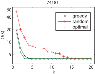
Figure 4 shows the effect of the different control policies. The greedy policy performs only slightly worse than the optimal policy, while the random policy needs more steps to reduce Ω(S). Note that we have chosen a smaller circuit so we can test the optimal control policy (|CTL| = 14, |IN| = 0).
In preparing the data for Fig. 4, the run-time of FRACTAL was negligible for the random and control policies (less than 3 s), while it took 43 min to compute the optimal control setting. Throughout our experiments we have established that the average run-time complexity of FRACTAL (including the time spent for diagnosis and consistency checking) is polynomial in |COMPS| and |CTL|, which makes FRACTAL applicable to large real-world systems.
6 Conclusions
We have described a novel approach, FRACTAL (FRamework for ACtive Testing ALgorithms), which, given an initial set of diagnoses computes an optimal sequence of additional test vectors for reducing the number of remaining diagnoses. At each step of testing, FRACTAL computes the test that maximally reduces the size of the existing diagnostic set. FRACTAL generates such test vectors using a greedy, next-best strategy, using a low-cost approximation of diagnostic information entropy to guide the search.
Extensive experimentation with ISCAS85 combinational circuits shows that FRACTAL reduces the number of remaining diagnoses according to a steep geometric decay function, even when only a fraction of inputs are available for active testing. Our experimental results indicate that FRACTAL's diagnostic convergence rate is close to optimal. This agrees with our theoretical claim that the approximate solution computed by FRACTAL's greedy approach is optimal over all poly-time approximation algorithms.
Acknowledgments
This work has been supported by STW grant DES.7015 and SFI grants 06-SRC-I1091 and 04-IN3-I524.
@inproceedings{ijcai2009p134,
  title     = {FRACTAL: Efficient Fault Isolation Using Active Testing},
  author    = {Feldman, Alexander and Provan, Gregory M. and van Gemund, Arjan J. C.},
  booktitle = {Proceedings of the Twenty-First International Joint Conference on
               Artificial Intelligence, {IJCAI-09}},
  publisher = {International Joint Conferences on Artificial Intelligence},
  editor    = {Craig Boutilier},
  pages     = {778--783},
  year      = {2009},
  url       = {https://ijcai.org/proceedings/2009/134},
}
TY - CPAPER TI - FRACTAL: Efficient Fault Isolation Using Active Testing AU - Feldman, Alexander AU - Provan, Gregory M. AU - van Gemund, Arjan J. C. T2 - Proceedings of the Twenty-First International Joint Conference on Artificial Intelligence, IJCAI-09 PB - International Joint Conferences on Artificial Intelligence PY - 2009 SP - 778 EP - 783 UR - https://ijcai.org/proceedings/2009/134 ER -Copied
Machine-readable versions of this paper, for tools and AI agents:





