Automated Benchmark Model Generators for Model-Based Diagnostic Inference

1 Diagnostic Inference for Complex Systems

Model-based diagnosis (MBD) focuses on determining whether an assignment of failure status to a set of modevariables is consistent with a system description and an observation (e.g., of sensor values). This problem is known to be NP-complete [Bylander et al., 1991; Friedrich et al., 1990]. However, this is a worst-case result, and some NP-complete problems, such as graph colouring [Cheeseman et al., 1991], are known to be tractable for particular problem classes.

We focus on the average-case complexity of MBD algorithms on real-world problem instances. At present, it is not known whether MBD is computationally difficult for the "average" system. There has been no systematic study of the complexity of diagnosing real-world problems, and few good benchmarks exist to test such a conjecture.

This article makes two main contributions. First, it describes an algorithm for automatically generating diagnostic benchmark models that can be used to analyse the performance of diagnostic inference algorithms. This model generator can be applied to any domain, and can generate models that accurately capture the properties of complex systems, given as input a library of domain-dependent component models. In particular, we propose a real-world graph model, that, given a model with n components, uses a small set of domain-dependent parameters to specify the complexity of diagnostic inference for a device. We compare the predictions made by our model to results obtained from ISCAS circuit benchmark models [Harlow, 2000]. By empirically comparing generated models with benchmark models we show the model-generation parameters best suited for ISCAS circuits. This approach circumvents the difficulty of assembling a large suite of test problems (benchmark models), given that most large diagnosis models tend to be proprietary. It also enables us to control model parameters (and hence analyse specific parameters).

∗Both authors are supported by SFI grant 04/IN3/I524.

Second, we use this framework to show empirically that diagnosing a suite of benchmark circuit models is computationally hard. This provides the first clear experimental demonstration of this computational intractability for a well-known benchmark suite.

We organize the remainder of the document as follows. Section 2 examines the topological structure that all realworld complex systems possess. Section 3 summarises the model-based diagnosis task that we solve. Section 4 describes the process we adopt for generating diagnostic models using domain parameters, and Section 5 describes the optimisation technique for auto-generation. Section 6 presents the experimental results, and Section 7 summarises our contributions.

2 Topological Models for Complex Systems

Several recent theoretical studies and extensive data analyses have shown that a variety of complex systems, including biological [Newman, 2003], social [Newman, 2003], and technological [Braha and Bar-Yam, 2004; i Cancho et al., 2001] systems, share a common underlying structure, which is characterised by a real-world graph. A real-world graph (RWG) is a complex network in which (a) the nodes form several loosely connected clusters, (b) every node can be reached from every other by a small number of hops or steps, and (c) the degree distribution P (k), which is the probability of finding a node with k links, follows a power-law [Newman, 2003].

Several random-graph models have been proposed to capture the real-world graph properties, such as the Watts- Strogatz (or small-world graph) and the Barabasi-Albert models [Newman, 2003]. In this article we adopt the smallworld graph (SWG) framework, whose key properties are summarised below. We assume that we have a graph G(V, E) with a set V of vertices and set E of edges. We assume that G is connected, i.e., there is a sequence of distinct edges (a path P) joining any two nodes in G. A graph is directed, i.e., called a digraph, if all its edges are directed. The degree of a vertex is the number of edges incident on that vertex.

The SWG framework addresses two graph parameters: mean distance L and clustering coefficient Θ. The mean distance L is the average of all distances, i.e., shortest paths connecting two vertices, in G. Graph clustering characterises the degree of cliquishness of a typical neighbourhood (a node's immediately connected neighbours). The clustering coefficient Θi for a vertex vi is the proportion of links between the vertices within its neighbourhood divided by the number of links that could possibly exist between them. The graph clustering coefficient is the average of the clustering coefficients for each vertex [Newman, 2003].

Several empirical studies, summarised in, e.g., [Newman, 2003], have shown that the SWG framework, with particular parameter settings, provides a good model for complex systems. These parameter settings are described in terms of random graph parameters as follows.

Definition 1 (SWG). A small-world-graph (SWG) is a graph G(V, E) that has small-world properties measurable in terms of its mean distance L and clustering coefficient Θ. Given a random graph G(n, p)1 with mean distance Lr, clustering coefficient Θr, and the same number of nodes and edges as G(V, E), a SWG has the properties L ≃ Lr and Θ ≫ Θr.

i Cancho et al. [2001] have applied real-world graphs to electronic circuits [i Cancho et al., 2001], mapping the vertices of the graph G to electronic components (gates, resistors, capacitors, diodes, etc.), and the edges of G to the wires between the components. The circuits studied comprise both analog and ISCAS89/ITC89 benchmark circuits, and all display Θ and L parameters that are typical of SWG topologies. In an electronic circuit, a cluster of components corresponds to components that together serve a particular task, e.g., a sub-system; the relatively small number of connections between clusters corresponds to the fact that sub-systems are typically loosely-coupled. In addition, the short paths between any pair of components (nodes) in a circuit are the natural result of wire-length minimisation typical of circuits.

3 Model-Based Diagnosis

We can characterise a MBD problem using the triple 〈COMPS, SD, OBS〉 [Reiter, 1987], where:

• COMPS = {C1, ...,Cm} describes the operating modes of the set of m components into which the system is decomposed.
• SD, or system description, describes the function of the system. This model specifies two types of knowledge,

1 The Erdos-Renyi G(n, p) model consists of n nodes, each pair of which is randomly connected with probability p, and has parameters (Lr,Θr) = ( ln(n) ln(pn) , p).

• denoted SD = (S, B), where S denotes the system structure (connections between the components), and B denotes the behaviour of the collection of components. 2
• OBS, the set of observations, denotes possible sensor measurements, which may be control inputs, outputs or intermediate variable-values.

We adopt a propositional logic framework for our system behaviour models B. Component i has associated modevariable Ci; Ci can be functioning normally ([Ci = OK]), or can take on a finite set of abnormal behaviours.

MBD inference assumes initially that all components are functioning normally: [Ci = OK], i = 1, ...,m. Diagnosis is necessary when SD ∪ OBS ∪ {[Ci = OK]|Ci ∈ COMPS} is proved to be inconsistent. Hypothesizing that component i is faulty means switching from [Ci = OK] to [Ci ̸= OK]. Given some minimality criterion ω, a (minimal) diagnosis is a (ω-minimal) subset C ′ ⊆ COMPS such that: SD ∪ OBS ∪ {[Ci = OK]|Ci ∈ COMPS \ C′} ∪ {[Ci ̸= OK]|Ci ∈ C′} is consistent.

In this article, we adopt a multi-valued propositional logic using standard connectives (¬, ∨, ∧,⇒). We denote variable A taking on value α using [A = α]. An example equation for a buffer X is [In = t] ∧ [X = OK] ⇒ [Out = t].

4 Benchmark Diagnostic Model Generation

This section describes our algorithm for generating benchmark diagnostic models. Figure 1 depicts the process of automatically generating diagnostic models and using them for evaluating diagnosis inference algorithms. Our approach is applicable to any domain, since (a) the underlying topological models can be tailored to virtually any complex system [Newman, 2003], and (b) functionality is incorporated into the system model using a component-library, where components can be developed for any domain in which the system models are decomposable.

The topology-generation method we adopt was originally developed based on the theory of random graphs-see [Newman, 2003] for background in this area. However, this method focuses solely on the system structure (as captured by the graph), and ignores the system functionality. We extend this approach by adopting the system structure based on the random-graph generators, and then encoding system functionality using a component library.

Model Generation Algorithm: We generate diagnostic (benchmark) models in a three-step process.

1. generate the (topology) graphGunderlying eachmodel;
2. assign components to each node in G for system SD, to create an MBD-graph G′ ;
3. generate the system description (and fault probabilities).

Every domain requires domain-specific parameters for generating realistic models. All real-world graph models require specific parameters to be able to match particular properties of a given domain [Costa et al., 2005]. For example, the SWGmodel requires specific parameters for initial graph connectivity k and random connectivity probability p; similarly, extended versions of the Barabasi-Albert model [Costa et al., 2005] need various parameters to capture properties such as inter-node distance and the cost of adding links. Analogous to these approaches, circuit auto-generation methods use domain-specific parameters like the Rent parameter ξ, e.g., [Verplaetse et al., 2000].

2S can be defined in several ways, such as through propositional sentences; in this article we define S in terms of a graph G(V, E).

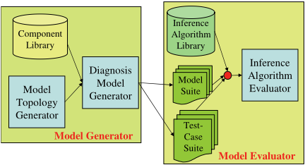
As an alternative to empirically-derived domain parameters that are known a priori, we can frame the generation task in terms of an optimisation task where we compute the domain parameters. The remainder of this section describes this auto-generation process based on domain-dependent parameters. We use an example, and then describe each step of the process. Section 5 describes the optimisation approach.

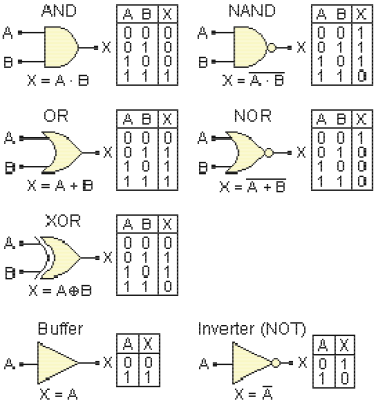
Example 1. To demonstrate this approach, we study a suite of auto-generated electronic combinational circuits, which are constructed from simple gates. The inputs to the generation process consist of: (a) a component library; (b) parameters defining the system properties, such as the number n of components; and (c) domain-dependent parameters, such as the well-known engineering parameter for determining input/output variables for a circuit, the Rent parameter ξ [Verplaetse et al., 2000]. As an example, Figure 2 shows several of the gates that we use in our component library, together with the gates' functionality (in terms of truth-tables).

Diagnosis models differ from generic circuit models in that they explicitly encode failure modes and the functional effect of failure modes. As a consequence, the structure of a diagnostic model is slightly different than the structure of the corresponding electronic circuit, since a diagnostic model explicitly encodes failure modes of components.

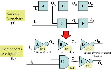
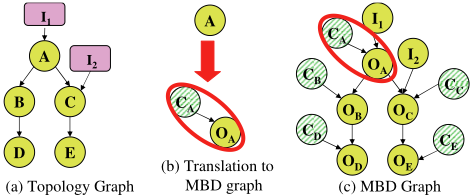
Example 2. Figure 3(a) shows the schematic of a simple circuit with arbitrary components A, B, C, D and E. The circuit has two inputs, I1 and I2, with the output of component i denoted by Oi. Figure 3(b) shows the circuit with instantiated components. Figure 4 shows the process of transforming this schematic into a MBD-graph, which is the basis for constructing a diagnostic model. We first translate the schematic into a topology graph, which makes the graphical topology of the circuit explicit by denoting each component as a node, the inputs as nodes, and the input-component and componentcomponent wires as directed edges. 3 Next we replace each component X in the topology graph with a pair (CX,OX), which denotes the mode and output of component X, respectively. We introduce the mode-variables for each component, and define component behavioural equations in order to diagnose the fault status of each component.

3 This is roughly the graphical framework used for the small-

The topology graph G and MBD-graph G′ are as follows. Definition 2 (Topology graph). A topology graph G(V,E) for a system 〈COMPS, SD,OBS〉 is a directed graph G(V,E) corresponding to the system structure S. Hence in G(V,E): (a) the nodes V consist of a collection of nodes corresponding to system components (χ), and system inputs (η), i.e., V = χ ∪ η; and (b) the edges correspond to connections between two component-nodes, or between an inputnode and a component-node, i.e., E = (χi, χj) ∪ (ηi, χk), for χi, χj , χk ∈ χ, and ηi ∈ η.

Definition 3 (MBD-graph). An MBD-graph G′ (V ′ , E′ ) is a topology graph G(V, E) in which each component node χi ∈ world analyses of electronic systems in [i Cancho et al., 2001].

V is replaced with a subgraph consisting of the node for the corresponding component-output Oi, the node corresponding to component-mode Ci, and the directed edge (Ci,Oi)-see Figure 4. Hence in G′ (V ′ , E′ ): (a) the nodes V ′ consist of a collection of nodes corresponding to system componentoutputs (O), mode-variables (COMPS), and system inputs (η), i.e., V = O ∪ COMPS ∪ η; and (b) the edges correspond to connections between two component-output-nodes, or between an input-node and a component-node, i.e., E = (Oi,Oj)∪(ηi,Ok)∪(Ci,Oi)), for Oi,Oj,Ok ∈ O, ηi ∈ η, and Ci ∈ COMPS.

4.1 Generate Graph Structure for G

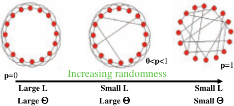
We generate a small-world-graph (SWG) using a revised version of the approach of Watts and Strogatz [Newman, 2003]. The SWG approach generates a graph G with a degree of randomness that is controlled by a probability p ∈ [0, 1]. p ≃ 0 corresponds to a regular graph, and p ≃ 1 corresponds to an Erdos-Renyi random graph; graphs with real-world structure (SWGs) occur in between these extremes, as has been determined by empirically comparing the Θ and L parameters of generated graphs and actual networks [Newman, 2003].

Figure 5 depicts the graph generation process, where we control the proportion of random edges using a rewiring probability p. Standard SWG generation takes a regular graph (a ring lattice of n nodes), where each node is connected to its k nearest neighbors, and randomly "rewires" an edge by moving one of its ends to a new position chosen at random (with probability p) from the rest of the lattice [Newman, 2003].

We have modified the SWG framework to enable us to match the mean degree of the graph for the ISCAS circuit with that of the generated graph, since the mean degree is a critical parameter in this framework. The original SWG model requires the mean degree k to be an even number; however, the mean degree in real circuits is typically not an integer. Our enhanced SWG generator first creates a ring lattice with degree k, where k is any positive real number, by setting k′ = ⌈ k2 ⌉, and connecting every node to its nearest k′ 2 neighbors on both sides, just as in the classic SWG model. Next it connects every node to its two k′ 2 + 1 nearest nodes on both sides, with probability (k-k′ ) 2 .

4.2 Assign Components to graph G

Given a topology graph G, we associate to each componentnode in G a component, based on the number of incoming arcs for the node. Given a SWG component-node with i inputs and o outputs, we assign a component, denoted SD(i, o, τ, B,w) where τ denotes the type (e.g., AND-gate, OR-gate), B defines the behavioural equations, and w the weights assigned to the failure modes.

Example 3. For our experiments, we use a set of digital comparator components, such as shown in Figure 2. Given a node that has q possible components that are suitable, we randomly select one with probability 1q . For example, the single-input nodes correspond to single-input gates (NOT, buffer), and the dual-input nodes correspond to dual-input gates (AND, OR, NAND, NOR, XOR), etc.

4.3 Generate the SystemDescription

Given a selected component, we then generate its normalmode equations (and potentially failure-mode equations). We randomly select the mode type (of the s possible failure modes) for any component-model with probability 1s . We assign weights to failure-mode values by assuming that normal behaviour is highly-likely, i.e., Pr{Ci = OK} ≃ 0.99, and faulty behaviour is unlikely, i.e., Pr{Ci ̸= OK} ≃ 0.01.

Example 4. Figure 3(b) shows a randomly-generated circuit based on the schematic of Figure 3(a). Here, we instantiate components A, D and E to NOT gates, component C to an AND gate, and component B to a buffer. This figure also depicts the instantiated failure-mode for the components in shaded boxes: Components B, C and E have SA1 faultmodes, component A has a SA0 fault-mode, and component D has a INVERT fault-mode. Given this information, we can generate a system description with equations corresponding to the component-types and fault-mode types as just described. For example, the equations for gates A and C are:

5 OptimisationModel-Generation Approach

This section reviews the optimisation approach we have adopted for generating the topology graph underlying realistic diagnosis models. The standard SWG generation process has a wide range of parameter choices, e.g., parameters

(n, k, p), that produce models with very different properties. Hence, one must generate a model using a parameter-setting that best captures a desired property. This approach is general, and can be used to create models for testing a variety of objectives, such as diagnostic inference complexity, model size, etc. Since we are generating models that can be used to test the relative efficiency of MBD inference algorithms, we pose the auto-generation problem as an optimisation problem whose objective function is defined in terms of the computational complexity of MBD inference.

MBD Auto-Generation Task: The objective of MBD auto-generation is to create a model SD that minimises |γA(SD, OBS) - γA(SD,OBS)|, where SD is an MBD model , and A is an MBD inference algorithm that has complexity γA(SD,OBS) when computing a ω-minimal diagnosis given model SD and observations OBS. 4

We have adopted the causal network approach [Darwiche, 1998] for our experiments. We used as our measure of inference complexity the largest clique-table in the compiled causal network model, which is a typical complexity measure for this type of model. The diagnosis minimality criterion ω is a order-of-magnitude probability function [Darwiche, 1998].

From a theoretical perspective, the complexity of causal network inference is expressed in terms of the graph topology: it is exponential in the largest clique of the graph (or the graph width) [Darwiche, 1998]. This indicates that the influence of behaviour B and observations OBS are outweighed by the graph structure.

We have shown experimentally that system structure is the primary determinant of diagnostic inference complexity for causal network diagnostic inference, i.e., γA(SD,OBS) ≃ γA(S). In particular, we showed that the diagnostic inference complexity was invariant to variation in the behaviour equations B and the observation set OBS. Using the structure of the ISCAS85 benchmark circuit C499, we examined 54 different combinations of component type and 6 sets of different observations. A two-way analysis of variance (ANOVA) of data averaged over 300 runs indicated that neither varying component types nor altering the number of observations had a statistically significant effect on the inference complexity. Hence we concluded that structure is the primary determinant of diagnostic inference complexity.

6 Experimental Comparison of Generated and ISCAS-Benchmark Models

This section summarises results of experiments comparing the structure and diagnostic inference complexity properties of auto-generated models with ISCAS benchmark models.

The ISCAS circuits are an established benchmark for circuit optimisation [Harlow, 2000]. The benchmark suites consist of multiple sets of circuits, of which we focus on the ISCAS85 combinational circuits. Our experiments were conducted on 3GHz Pentium-IV with 3GB of RAM. All data presented is based on an average of 300 runs. Given an ISCAS circuit SD with n components, we generated a diagnostic SWG model SD with n nodes, by varying the graphgeneration parameters (k, p) in order to choose the best parameter setting such that SD and SD had the same diagnostic performance.

4 We assume that γ(·) returns a complexity parameter such as CPU-time or number of nodes searched.

6.1 Average-Case Diagnosis Complexity

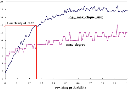
Our first set of experiments explored the complexity of autogenerated models corresponding to all ISCAS85 circuits over the entire range of the rewiring parameter p. Figure 6 shows the maximal degree of the generated graph G (corresponding to C432) compared with the log10 of the inference complexity of G. The figure shows that both curves have the same trend, rising from the relatively efficient regular graph (p = 0) to the range of small-world graphs (0 > p > 1). This increase occurs because, given a graph with n nodes, a SWG will have more and larger clique-tables than a regular graph,and hence will be computationally harder than a regular graph.

Given that all circuits demonstrated properties similar to those shown in Figure 6, i.e., complexity exponential in the largest clique (or intractability for non-trivial circuits), our experiments have shown that the ISCAS85 circuits are computationally difficult to diagnose, on average.

6.2 Parameter Optimisation

We then studied two approaches to choosing parameters that minimise the diagnosis-complexity difference between ISCAS and generated circuits: matching topological parameters governing (1) degree distribution, k, an easily-computed topological parameter; and (2) diagnostic complexity, γA, a computationally intensive measure.

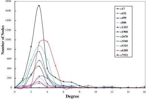
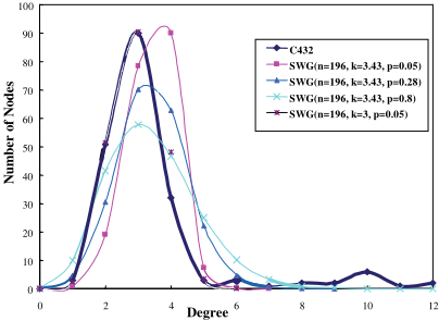
Degree Distribution: We first tried to match the diagnostic complexity of corresponding models SD and SD by matching the degree distributions of SD and SD. Figure 7 shows the degree distributions of ISCAS85 circuits. For each real circuit most nodes have low degree; however, each graph in Figure 7 also has a long tail containing some high-degree nodes that significantly affect the inference complexity, since the complexity is proportional to the node of highest degree. A generated SWG has a unimodal degree distribution that matches the most-likely degrees very well, but not the tail of the curve. For example, consider the SWG for C432, with

(n = 196, k = 3, p = 0.05), whose degree distribution is shown in Figure 8; this SWG contains fewer edges than C432, and our experiments indicate that its inference complexity is also much lower than that of C432. Obviously, just matching the most-likely degree does not lead to generated models that match the complexity of ISCAS85 circuits due to the absence of long tails.

Inference-Complexity Optimisation: Next, we set the mean degree of SD to be that of the real circuit SD, and experimentally selected the rewiring probability p that minimised |γA(SD, OBS) -γA(SD, OBS)| over a broad range of observations. As shown in Figure 8, increasing p (for fixed k) modifies the SWG degree distribution by flattening the distribution, lowering the magnitude of the peak value but increasing the length of the tail (and hence increasing the inference complexity of SD). For example, empirical comparisons showed that the SWG with (n = 196, k = 3.43, p = 0.28) produced a model with inference complexity closest to that of C432-see Figure 6. In our experiments we found that the ISCAS85 circuits all had corresponding SWG models with p < 0.3. 5 Note that p < 0.3 corresponds to SWG models of relatively low complexity, i.e., we can generate models of significantly higher complexity than the ISCAS85 circuits, thus providing a range of difficulty of auto-generated models.

7 Conclusion

This article has described a method for generating diagnostic models that have real-world topology and can be tailored to different domains. We have generated models of systems composed of digital circuits, but can generalise this approach to any domain where systems can be composed from a library of components. This method circumvents the problems with using random-graphs for experiments, and provides an alternative to developing suites of hand-built benchmark models. This article has also empirically shown that MBD problems with a real-world topology, i.e., with a SWG structure, are computationally hard.

5 It is interesting to note that our auto-generated circuits had an effective Rent parameter similar to that of the original circuits, indicating the correctness of the approach.