First Order Decision Diagrams for Relational MDPs

1 Introduction

In the past years there has been an increased interest in developing relational or first order MDPs. Some examples include symbolic dynamic programming (SDP) [Boutilier et al., 2001], the relational Bellman algorithm (ReBel) [Kersting et al., 2004], approximate linear programming for FOMDPs [Guestrin et al., 2003; Sanner and Boutilier, 2005], approximate policy iteration [Fern et al., 2003], and inductive policy selection using first order regression [Gretton and Thiebaux, 2004].

Among these, only SDP and ReBel are exact solution methods. To our knowledge there is no working implementation of SDP because it is hard to keep the state formulas consistent and of manageable size in the context of situation calculus. Compared with SDP, ReBel provides a more practical solution. ReBel uses simpler language (a probabilistic STRIPS-like language) to represent FOMDPs, so that reasoning over formulas is easier to perform.

Inspired by the successful application of Algebraic Decision Diagrams (ADD) [Bryant, 1986; Bahar et al., 1993] in solving propositionally factored MDPs [Hoey et al., 1999; St-Aubin et al., 2000] we lift propositional ADDs to handle relational structure and use them in the solution of FOMDPs. The intuition behind this idea is that the ADD representation allows information sharing, e.g., sharing between state partitions. If there is sufficient regularity in the model, ADDs can be very compact, allowing problems to be represented and solved efficiently.

First order decision trees and even decision diagrams have already been considered in the literature [Blockeel and De Raedt, 1998; Groote and Tveretina, 2003] and several semantics for such diagrams are possible. In particular Groote and Tveretina [2003] provide a notation for first order BDDs that can capture formulas in Skolemized conjunctive normal form and then provide a theorem prover based on this representation. In this paper we adapt and extend their approach to handle first order MDPs. In particular, we extend the definitions to handle existential quantification and numerical leaves through the use of an aggregation function. This allows us to capture value functions using algebraic diagrams in a natural way. We also provide additional reduction transformations for algebraic diagrams that help keep their size small, and allow the use of background knowledge in reductions. We then develop appropriate representation and algorithms showing how value iteration can be performed using the decision diagrams.

It is useful to compare our solutions to the propositional ones. The main difficulty in lifting the ideas is that in relational domains the transition function specifies schemas for conditional probabilities. The propositional solution uses the concrete conditional probability to calculate the regression function. But this is not possible with schemas. While one can first ground the domain and problem at hand and only then perform the reasoning (e.g. [Sanghai et al., 2005]) this does not allow for solutions abstracting over domains and problems. Like SDP and ReBel our constructions do perform general reasoning and they do so by using decision diagrams.

Due to space constraints most proofs and some details are omitted from the paper.

2 Markov Decision Processes

We assume familiarity with standard notions of MDPs and value iteration [Puterman, 1994]. In the following we introduce some of the notions and our notation. A MDP can be characterized by a state space S, an action space A, a state transition function Pr(sj|si, a) denoting the probability of transition to state sj given state si and action a, and an immediate reward function r(s), specifying the immediate utility of being in state s. A solution to a MDP is an optimal policy that maximizes expected discounted total reward as defined by the Bellman equation. The value iteration algorithm uses the Bellman equation to iteratively refine an estimate of the value function:

where Vn(s) represents our current estimate of the value function and Vn+1(s) is the next estimate.

The main observation used by Hoey et al. [1999] is that if we can represent each of r(s), Pr(s′ |s, a), and Vk(s) compactly using ADDs then value iteration can be done directly using this representation, avoiding the need to enumerate the state space which is implicit in the equation above.

Taking the next step, the SDP approach [Boutilier et al., 2001] was developed in the context of the situation calculus. Stochastic actions are specified as a non-deterministic choice among deterministic alternatives. In this way one can separate the regression over action effects, which is now deterministic, from the probabilistic choice of action. On each regression step during value iteration, the value of a stochastic action A(⃗x) parameterized with free variables ⃗x is determined in the following manner:

where rCase(s) and vCase(s) denote reward and value functions in the compact "case notation" of Boutilier et al. [2001], nj(⃗x) denotes the possible outcomes of A(⃗x), and pCase(nj(⃗x), s) the choice probabilities for nj(⃗x).

After the regression, we need to maximize over the action parameters of each Q-function to get the maximum value that could be achieved by using an instance of this action. In SDP, this is done by adding the negation of higher value partitions into the description of lower value partitions, leading to complex formulas and reasoning. Finally, to get the next value function we maximize over the choice of action.

The solution of ReBel [Kersting et al., 2004] follows the same outline but uses a probabilistic STRIPS-like language for representing FOMDPs. More importantly the paper uses a decision list [Rivest, 1987] style representation for value functions. The decision list gives us an implicit maximization operator since rules higher on the list are evaluated first. As a result the object maximization step is very simple. On the other hand regression in ReBel requires that one enumerate all possible matches between a subset of a state partition and action effects and reason about each of these separately.

3 First Order Decision Diagrams

An Algebraic Decision Diagram is a labeled directed acyclic graph where non-leaf nodes are labeled with propositional variables, each non-leaf node has exactly two children corresponding to true and false branches, and leaves are labeled with numerical values. Ordered decision diagrams specify a fixed order on propositions and require that node labels respect this order on every path in the diagram. In this case every function has a unique canonical representation and diagrams have efficient manipulation algorithms, leading to successful applications [Bryant, 1986; Bahar et al., 1993].

There are various ways to generalize ADDs to capture relational structure. One could use closed or open formulas in the nodes, and in the latter case we must interpret the quantification over the variables. We focus on the following syntactic definition which does not have any explicit quantifiers.

Definition of First Order Decision Diagrams:

1. We assume a signature with a fixed set of predicates and constant symbols, and an enumerable set of variables. We also allow to use an equality between any pair of terms (constants or variables).

(2) A First Order Decision Diagram (FODD) is a labeled directed acyclic graph, where each non-leaf node has exactly two children. The outgoing edges are marked with values true and false.

1. Each non-leaf node is labeled with: an atom P (t1, . . . , tn) or an equality t1 = t2 where ti is a variable or a constant.

(4) Leaves are labeled with numerical values.

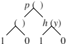
Figure 1 shows a FODD with binary leaves. Left going edges represent true branches. To simplify diagrams in the paper we draw multiple copies of the leaves 0 and 1 but they represent the same node in the FODD.

The semantics of first order formulas are given relative to interpretations. An interpretation has a domain of elements, a mapping of constants to domain elements, and for each predicate a relation over the domain elements which specifies when the predicate is true. There is more than one way to define the meaning of FODD B on interpretation I. In the following we discuss two possibilities.

Semantics based on a single path: A semantics for decision trees is given by Blockeel and De Raedt [1998] that can be adapted to FODDs. The semantics define a unique path that is followed when traversing B relative to I. All variables are existential and a node is evaluated relative to the path leading to it. For example, if we evaluate the diagram in Figure 1 on the interpretation I1 with domain {1, 2, 3} and relations {p(1), q(2), h(3)} then we follow the true branch at the root since ∃x, p(x) is satisfied, but we follow the false branch at q(x) since ∃x, p(x) ∧ q(x) is not satisfied. Since the leaf is labeled with 0 we say that B does not satisfy I. This is an attractive approach, since it builds mutually exclusive partitions over states, and various FODD operations can be developed for it. However, for reasons we discuss later this semantics is not well suited to value iteration, and it is therefore not used in the paper.

Semantics based on a multiple paths: FollowingGroote and Tveretina [2003] we define the semantics first relative to a variable valuation ζ. Given a FODD B over variables ⃗x and an interpretation I, a valuation ζ maps each variable in ⃗x to a domain element in I. Once this is done, each node predicate evaluates either to true or false and we can traverse a single path to a leaf. The value of this leaf is denoted by MAPB(I, ζ).

We next define MAPB(I) = aggregateζ {MAPB(I, ζ)} for some aggregation function. That is, we consider all possible valuations ζ, for each we calculate MAPB(I, ζ) and then we aggregate over all these values. In [Groote and Tveretina, 2003] leaf labels are in {0, 1} and variables are universally quantified; this is easily captured by using minimum as the aggregation function. In this paper we use maximum as the aggregation function. This corresponds to existential quantification in the binary case, and gives useful maximization for value functions in the general case. We therefore define: MAPB(I) = maxζ {MAPB(I , ζ)}.

Consider evaluating the diagram in Figure 1 on the interpretation I1. The valuation {x/2, y/3} leads to a leaf with value 1 so the maximum is 1 and we say that I satisfies B.

We define node formulas (NF) and edge formulas (EF) recursively as follows. For a node n labeled l(n) with incoming edges e1, . . . , ek, the node formula NF(n) = (∨iEF(ei)). Denote the true branch of a node n by n↓t and the false branch by n↓f . The edge formula for the true outgoing edge of n is EF(n↓t) = NF(n) ∧ l(n). The edge formula for the false outgoing edge of n is EF(n↓f) = NF(n)∧¬l(n). These formulas, where all variables are existentially quantified, capture reachability conditions for the node or edge.

Basic Reduction of FODDs: Groote and Tveretina [2003] define several operators that reduce a diagram into "normal form". A total order over open predicates (node labels) is assumed. We describe these operators briefly and give their main properties.

(R1) Neglect operator: if both children of a node p in the FODD lead to the same node q then we remove p and link all parents of p to q directly. (R2) Join operator: if two nodes p, q have the same label and point to the same two children then we can join p and q (remove q and link q's parents to p). (R3) Merge operator: if a node and its child have the same label then the parent can point directly to the grandchild. (R4) Sort operator: If a node p is a parent of q but the label ordering is violated (l(p) > l(q)) then we can reorder the nodes locally using two copies of p and q such that labels of the nodes do not violate the ordering.

Define a FODD to be reduced if none of the four operators can be applied. We have the following:

Theorem 1 [Groote and Tveretina, 2003]

(1) Let O ∈ {Neglect, Join, Merge, Sort} be an operator and O(B) the result of applying O to FODD B, then for any ζ, MAPB(I, ζ) = MAPO(B)(I, ζ)

(2) if B1,B2 are reduced and satisfy ∀ζ, MAPB1 (I, ζ) = MAPB2 (I, ζ) then they are identical.

Property (1) gives soundness, and property (2) shows that reducing a FODD gives a normal form. This only holds if the maps are identical for every ζ and this condition is stronger than normal equivalence. However, this weak normal form suffices for Groote and Tveretina [2003] who use it to provide a theorem prover for first order logic.

Combining FODDs: Given two algebraic diagrams we may need to add the corresponding functions, take the maximum or use any other binary operation op over the values represented by the functions. Here we adopt the solution from the propositional case [Bryant, 1986] in the form of the procedure Apply(p, q, op) where p and q are the roots of two diagrams. This procedure chooses a new root label (the lower among labels of p, q) and recursively combines the corresponding sub-diagrams, according to the relation between the two labels (<, =, or >).

Additional Reduction Operators: In our context, especially for algebraic FODDs we may want to reduce the diagrams further. We distinguish strong reduction that preserves MAPB(I, ζ) for all ζ and weak reduction that only preserves MAPB(I). In the following let B represent any background knowledge we have about the domain. For example in the Blocks World we may know that ∀x, y, [on(x, y) → ¬clear(y)].

(R5) Strong Reduction for Implied Branches: Consider any node n with label l(n). Let ⃗x be the variables in EF(n↓t). If B |= ∀⃗x, [NF(n) → l(n)] then whenever node n is reached then the true branch is followed. In this case we can remove n and connect its parent directly to the true branch. It is clear that the map is preserved for any valuation. A similar reduction can be formulated for the false branch.

(R6) Weak Reduction Removing Dominated Siblings: Consider any node n such that if we can reach n we can also reach n↓t. If n↓t always gives better values than n↓f then we should be able to remove n↓f from the diagram. We start by giving a special case of this condition.

Let ⃗x be the variables that appear in NF(n), and ⃗y the variables in l(n) and not in NF(n). Consider the condition (I1): B |= ∀⃗x, [NF(n) → ∃⃗y, l(n)] which requires that every valuation reaching n can be extended to reach n↓t.

Let min(n↓t) be the minimum leaf value in n↓t, and max(n↓f ) be the maximum leaf value in n↓f . Consider next the additional condition (V1): min(n↓t) ≥ max(n↓f). In this case regardless of the valuation we know that it is better to follow n↓t and not n↓f . If both I1 and V1 hold then according to maximum aggregation the value of MAPB(I) will never be determined by the false branch. Therefore we can safely replace n↓f with any constant value between 0 and min(n↓t) without changing the map. A symmetric operation can be applied exchanging the roles of n↓t and n↓f .

In some cases we can also drop the node n completely and connect its parents directly to n↓t. This can be done if (I1A): B |= ∀⃗u, [∃⃗v,NF(n)] → [∃⃗v, ⃗w, EF(n↓t)] where ⃗u are the variables that appear in (the sub-diagram of) n↓t, ⃗v the variables that appear in NF(n) but not in n↓t, and ⃗w the variables in l(n) and not in ⃗u or ⃗w. This condition requires that for every valuation ζ1 that reaches n↓f there is a valuation ζ2 that reaches n↓t and such that ζ1 and ζ2 agree on all variables in n↓t. It is easy to see that I1A follows from I1 if (I1B): no variable in ⃗y appears in the sub-diagram of n↓t.

An important special case of R6 occurs when l(n) is an equality t1 = y where y is a variable that does not occur on the FODD above node n. In this case, the condition I1 holds since we can choose the value of y. Therefore if V1 holds we can remove the node n connecting its parents to n↓t and substituting t1 for y in the diagram n↓t.

(R6) General Case: The conditions for replacing n↓f with a constant and for dropping n completely can be relaxed. Due to space constraints, we only sketch the details. I1 can be relaxed to (I2): B |= [∃⃗x, NF(n)] → [∃⃗x, ⃗y, EF(n↓t)], which requires that if n is reachable then n↓t is reachable but does not put any restriction on the valuations (in contrast with I1).

Let D = n↓t - n↓f which we can calculate using Apply. V1 can be relaxed to (V2): all leaves in D have non-negative values. But using V2 requires a condition stronger than I2.

(R7) Weak Reduction Removing Dominated Edges:

Consider a FODD with two nodes p, q where q is in the sub-FODD of p↓f and their formulas satisfy that if we can follow q↓t then we can also follow p↓t. In this case, if min(p↓t) ≥ max(q↓t) then MAPB(I) will never be determined by q↓t so we can replace q↓t with a constant between 0 and min(p↓t). If in addition we have min(p↓t) ≥ max(q↓f ) then it is also safe to remove q completely. Due to space constraints, we omit the details and the general case of R7.

(R8) Weak Reduction by Unification: Consider a FODD B and two sets of variables ⃗x and ⃗y of the same cardinality. By B{⃗x/⃗y} we denote the FODD resulting from replacing variables in ⃗x by the corresponding variables in ⃗y. Now consider the FODD B{⃗x/⃗y} - B which we can calculate using Apply. If all leaves in this diagram are non negative then ∀I, MAPB(I) = MAPB{⃗x/⃗y}(I) so we can safely replace B.

4 Decision Diagrams for MDPs

We follow Boutilier et al. [2001] and specify stochastic actions as a non-deterministic choice among deterministic alternatives. We therefore need to use FODDs to represent the deterministic domain dynamics of actions, the probabilistic choice among actions, and value functions.

Example Domain: We use the logistics problem variant from [Boutilier et al., 2001] to illustrate our constructions for MDPs. The domain includes boxes, trucks and cities, and predicates are Bin(Box, City), T in(T ruck, City), and On(Box, Truck) with their obvious meaning. The reward function, capturing a planning goal, awards a reward of 10 if the formula ∃b,Bin(b, Paris) is true, that is if there is any box in Paris.

The domain includes 3 actions load, unload, and drive. Actions have no effect if their preconditions are not met. Actions can also fail with some probability. When attempting load, a successful version loadS is executed with probability 0.99, and an unsuccessful version loadF (effectively a nooperation) with probability 0.01. The drive action is executed deterministically. When attempting unload, the probabilities depend on whether it is raining or not. If it is not raining (raining) then unloadS is executed with probability 0.9 (0.7), and unloadF with probability 0.1 (0.3).

The domain dynamics: are defined by truth value diagrams (TVDs). For every action schema A(⃗a) and each predicate schema p(⃗x) the TVD T(A(⃗a), p(⃗x)) is a FODD with {0, 1} leaves. The TVD gives the truth value of p(⃗x) in the next state when A(⃗a) has been performed in the current state. We call ⃗a action parameters, and ⃗x predicate parameters. No other variables are allowed in the TVD.

Notice that the TVD simultaneously captures the truth values of all instances of p(⃗x) in the next state. Notice also that TVDs for different predicates are separate and independent. This can be safely done even if an action has correlated effects (not conditionally independent) since the actions are deterministic.

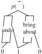
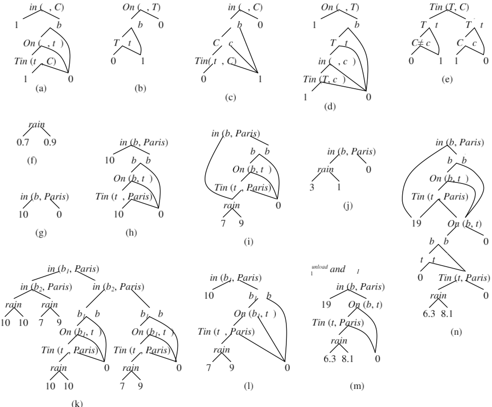
For any domain, a TVD for predicate p(⃗x) can be defined generically as in Figure 2. The idea is that the predicate is true if it was true before and is not "undone" by the action or was false before and is "brought about" by the action. TVDs for the logistics domain in our running example are given in Figure 3. All the TVDs omitted in the figure are trivial in the sense that the predicate is not affected by the action. In order to simplify the presentation we give the TVDs in their generic form and did not sort the diagrams.

Notice how we utilize the multiple path semantics with maximum aggregation. A predicate is true if it is true according to one of the paths specified so we get a disjunction over the conditions for free. If we use the single path semantics then a single path in a TVD must capture all possibilities for a predicate to become true in a state. Thus different conditions must be tested sequentially and their bindings must be combined so the corresponding notion of TVD is significantly more complicated.

Probabilistic Action Choice: Multiple path semantics makes it hard to specify mutually exclusive conditions using existentially quantified variables and in this way specify a distribution. We therefore restrict the conditions to be either propositional or depend directly on the action parameters. Notice that under this restriction any interpretation follows exactly one path (since there are no variables and thus only the empty valuation) so the aggregation function does not interact with the probabilities assigned. A diagram showing the choice probability for unloadS in our logistics example is given in Figure 3.

Reward and value functions: can be represented directly using algebraic FODDs. An example is given in Figure 3.

5 Value Iteration with FODDs

The general first order value iteration algorithm works as follows: given as input the reward function R and the action model, we set V0 = R, n = 0 and perform the following steps until termination:

1. For each action type A(⃗x), compute:

T A(⃗x) n+1 (Vn) = ⊕j (prob(Aj (⃗x)) ⊗ Regr(Vn, Aj (⃗x))).

1. QAn+1 = R ⊕ [γ ⊗ obj-max(T A(⃗x) n+1 (Vn))].

(3) Vn+1 is obtained by maximizing over Qn+1:

• Vn+1 = maxA QAn+1.

Regression by Block Replacement: Consider Vn and the nodes in its FODD. For each such node take a copy of the corresponding TVD, where predicate parameters are renamed so that they correspond to the node's arguments and action parameters are unmodified. Block Replacement Regression BR-regress(Vn, Aj (⃗x)) is the FODD resulting from replacing each node in Vn with the corresponding TVD, with outgoing edges connected to the 0, 1 leaves of the TVD. One can show that block replacement preserves the map for any valuation w.r.t. corresponding states.

However, naive implementation of block replacement may not be efficient. If we use block replacement for regression then the resulting FODD is not necessarily reduced or sorted. Reducing and sorting the results may be an expensive operation. Instead we calculate the result as follows. We traverse Vn using postorder traversal, where in the recursive step we combine the TVD block of the corresponding node (which is a TVD with binary leaves) with the processed versions of its children (which are general FODDs). If we call the parent B, the true branch child Bt and the false branch childBf then their combination is equivalent to [B×Bt]+[(1-B)×Bf ]. The result can be calculated by several calls to the Apply procedure. We can use strong reduction during block combination; weak reductions can only be applied after all blocks have been combined.

Object Maximization: As mentioned above we get maximization over action parameters for free. We simply rename the action parameters using new variable names (to avoid repetition between iterations) and consider them as variables. The aggregation semantics provides the maximization. Since constants are turned into variables additional reduction is typically possible at this stage. Any combination of weak and strong reductions can be used.

Adding and Maximizing Over Actions: These can be done directly using the Apply procedure. Recall that prob(Aj(⃗x)) is restricted to include only action parameters and cannot include variables. We can therefore calculate prob(Aj(⃗x)) ⊗ Regr(Vn,Aj(⃗x)) in step (1) directly. However, the different regression results are independent functions so that in the sum ⊕j(prob(Aj (⃗x))⊗Regr(Vn, Aj (⃗x))) we must standardize apart the different regression results before adding the functions (note that action parameters are still considered constants at this stage). Similarly the maximization Vn+1 = maxAQAn+1 in step (3) must first standardize apart the different diagrams. The need to standardize apart complicates the diagrams and often introduces structure that can be reduced. In each of these cases we first use the propositional Apply procedure and then follow with weak and strong reductions.

Figure 3 traces several steps in the application of value iteration to the logistics domain. In order to simplify the presentation the diagrams are not completely sorted allowing equalities in arbitrary locations.

6 Discussion

ADDs have been used successfully to solve propositional factored MDPs. Our work gives one proposal of lifting these ideas to FOMDPs. While the general steps are similar the technical details are significantly more involved than the propositional case. It is easy to see that our approach can capture probabilistic STRIPS style formulations as in ReBel, allowing for more flexibility in representation. However, it is more limited than SDP since we cannot use arbitrary formulas for rewards, transitions, and probabilistic choice (e.g. no universal quantification).

An implementation and empirical evaluation are obvious next steps. Also it would be interesting to investigate conditions that guarantee a normal form for a useful set of reduction operators, and improvements of the representation to achieve further compression.

Acknowledgments

This work has been partly supported by NSF Grant IIS-0099446, and by a Research Semester Fellowship Award from Tufts University.