
Ensembles of Partially Trained SVMs with Multiplicative Updates
Proceedings of the Twentieth International Joint Conference on Artificial Intelligence. Pages 1089-1093.
© 2007 International Joint Conferences on Artificial Intelligence
Abstract
The training of support vector machines (SVM) involves a quadratic programming problem, which is often optimized by a complicated numerical solver. In this paper, we propose a much simpler approach based on multiplicative updates. This idea was first explored in [Cristianini et al., 1999], but its convergence is sensitive to a learning rate that has to be fixed manually. Moreover, the update rule only works for the hard-margin SVM, which is known to have poor performance on noisy data. In this paper, we show that the multiplicative update of SVM can be formulated as a Bregman projection problem, and the learning rate can then be adapted automatically. Moreover, because of the connection between boosting and Bregman distance, we show that this multiplicative update for SVM can be regarded as boosting the (weighted) Parzen window classifiers. Motivated by the success of boosting, we then consider the use of an adaptive ensemble of the partially trained SVMs. Extensive experiments show that the proposed multiplicative update rule with an adaptive learning rate leads to faster and more stable convergence. Moreover, the proposed ensemble has efficient training and comparable or even better accuracy than the best-tuned soft-margin SVM.
- [Collins and Schapire, 2002] M. Collins and R.E. Schapire. Lo- gistic regression, AdaBoost and Bregman distances. Machine Learning, 48(1/2/3), 2002.
- [Cristianini et al., 1999] N. Cristianini, C. Campbell, and J. Shawe- Taylor. Multiplicative updatings for support vector machines. In Proceeding of European Symposium on Artificial Neural Net- works, Bruges, Belgium, 1999.
- [Evgeniou et al., 2004] T. Evgeniou, M. Pontil, and A. Elisseeff. Leave one out error, stability, and generalization of voting com- binations of classifiers. Machine Learning, 55(1):71-97, April 2004.
- [Fedotov et al., 2001] A.A. Fedotov, P. Harremoes, and F. Topsoe. Vajda's tight lower bound and refinements of Pinsker's inequality. In Proceedings of the International Symposium on Information Theory, San Mateo, CA, 2001.
- [Fine and Scheinberg, 2001] S. Fine and K. Scheinberg. Efficient SVM training using low-rank kernel representations. Journal of Machine Learning Research, 2:243-264, December 2001.
- [Hastie et al., 2005] T. Hastie, S. Rosset, R. Tibshirani, and J. Zhu. The entire regularization path for the support vector machine. In Lawrence K. Saul, Yair Weiss, and Léon Bottou, editors, Ad- vances in Neural Information Processing Systems 17, pages 561- 568. MIT Press, Cambridge, MA, 2005.
- [Kim et al., 2003] H.-C. Kim, S. Pang, H.-M. Je, D. Kim, and S. Bang. Constructing support vector machine ensemble. Pat- tern Recognition, 36(12):2757-2767, 2003.
- [Kivinen and Warmuth, 1997] J. Kivinen and M.K. Warmuth. Ad- ditive versus exponentiated gradient updates for linear prediction. Information and Computation, 132(1):1-64, 1997.
- [Kivinen and Warmuth, 1999] J. Kivinen and M. K. Warmuth. Boosting as entropy projection. In Proceedings of the Twelfth Annual Conference on Computational Learning Theory, pages 134 -144, Santa Cruz, CA, USA, 1999.
- [Lin, 2001] C.-J. Lin. Linear convergence of a decomposition method for support vector machines. Technical report, National Taiwan University, 2001.
- [Platt, 1999] J.C. Platt. Fast training of support vector machines us- ing sequential minimal optimization. In B. Schölkopf, C. Burges, and A. Smola, editors, Advances in Kernel Methods -Support Vector Learning, pages 185-208. MIT Press, Cambridge, MA, 1999.
- [Rätsch and Warmuth, 2005] G Rätsch and M Warmuth. Efficient margin maximization with boosting. Journal of Machine Learn- ing Research, 6:2131-2152, 2005.
- [Rätsch, 2001] G. Rätsch. Robust Boosting via Convex Optimiza- tion: Theory and Applications. PhD thesis, University of Pots- dam, October 2001.
References were extracted automatically from the PDF and may contain errors.
Full text extracted automatically from the PDF; figures, tables and equations may differ. The PDF is the version of record.
1 Introduction
Kernel methods, such as the support vector machines (SVMs), have been highly successful in many machine learning problems. Standard SVM training involves a quadratic programming (QP) problem, which is often solved by a complicated numerical solver. Moreover, while a general-purpose QP solver can be used, they are inefficient on this particular type of QPs. Consequently, a lot of specialized optimization techniques have been developed. The most popular approach is by using decomposition methods such as sequential minimization optimization (SMO) [Platt, 1999], which involves sophisticated working set selection strategies, advance caching schemes for the kernel matrix and its gradients, and also heuristics for stepsize prediction.
A much simpler approach is to use multiplicative updates, which was first explored in [Cristianini et al., 1999]. However, its convergence is sensitive to a learning rate that has to be fixed manually. When the learning rate is too large, overshooting and oscillations occur; while when it is too small, convergence is slow.
A second problem with the multiplicative update rule is that it can only work with the hard-margin SVM. However, on noisy data, the hard-margin SVM has poor performance and the soft-margin SVM, which can trade off complexity with training error, is usually preferred. However, the choice of this tradeoff parameter, which can be from zero to infinity, is sometimes critical. Various procedures have been proposed for its determination, such as by using cross-validation or some generalization error bounds [Evgeniou et al., 2004]. However, they are typically very computationally expensive.
Another possibility that avoids parameter tuning completely is by using the ensemble approach. [Kim et al., 2003] combines multiple SVMs with different parameters, and obtains improved performance. However, as a lot of SVMs still have to be trained, this approach is also very expensive.
In this paper, we first address the learning rate problem by formulating the multiplicative update of SVM as a Bregman projection problem [Collins and Schapire, 2002]. It can then be shown that this learning rate can be adapted automatically based on the data. Moreover, because of the connection between boosting and Bregman distance [Collins and Schapire, 2002; Kivinen and Warmuth, 1999], we show that this multiplicative update can be regarded as a boosting algorithm in which the (weighted) Parzen window classifiers are the base hypotheses, and each base hypothesis added to the ensemble is a partially trained hard-margin SVM. Now, in the boosting literature, it is well-known that the whole ensemble performs better than a single base hypothesis. Hence, to address the possibly poor performance of the hard-margin SVM, we consider using the whole ensemble of partially trained SVMs for prediction. Note that this comes at little extra cost in the multiplicative updating procedure. Experimentally, this ensemble is observed to have comparable or even better accuracy than the best-tuned soft-margin SVM.
The rest of this paper is organized as follows. The learning rate problem in multiplicative update is addressed in Section 2. The connection between this update process and boosting, together with the proposed ensemble of partially trained hard-margin SVMs, is then discussed in Section 3. Experimental results are presented in Section 4, and the last section gives some concluding remarks.
2 Multiplicative Updating Rule of SVM
In this paper, we focus on a particular variant of the hardmargin SVM, called ρ-SVM in the sequel, which will be introduced in Section 2.1. We then develop in Sections 2.2 and 2.3 an iterative multiplicative updating procedure based on the Bregman projection [Collins and Schapire, 2002; Kivinen and Warmuth, 1999]. The convergence of this iterative procedure is shown in Section 2.4.
2.1 Hard-Margin ρ-SVM
Given a training set {xi, yi}mi=1 , where xi ∈ Rd and yi ∈ R, the ρ-SVM finds the plane f (x) = w′ϕ(x) in the kernelinduced feature space (with feature map ϕ) that separates the two classes with maximum margin ρ/‖w‖:
The corresponding dual is:
where 0 and 1 are vectors of zero and one respectively, α = [α1, . . . , αm]′ is the vector of Lagrange multipliers, and ˜K = [yiyjk(xi, xj)]. It can be easily shown that
Because of the zero duality gap, the objectives in (1) and (2) are equal at optimality 1 , i.e.,
Denote
where ¯ ρ is the Lagrangian multiplier for the dual constraint α′1 = 1. Moreover, the Karush-Kuhn-Tucker (KKT) conditions lead to:
where ⊥ denotes that the two vectors are orthogonal, and
on using (3). Moreover, the optimal ¯ ρ (i.e., the dual variable of the dual) is indeed equal to the optimal primal variable ρ:
1 Here, variables at optimality are denoted by the superscript ∗ .
2.2 Bregman Projection
In this section, we assume that we have access to the optimal value of ρ∗ . We will return to the issue of determining ρ∗ in Section 2.3.
As α ∈ Pm = {α ∈ Rm | α ≥ 0, α′1 = 1}, the mdimensional probability simplex, a natural choice of the Bregman distance is the (unnormalized) relative entropy. At the tth iteration, we minimize the Bregman distance between the new α and the current estimate αt = [α(t) 1 , . . . , α(t) m ]′ , while requiring α to satisfy α′ ∂u(αt,ρ∗ ) ∂α = α′ ( ˜Kαt - ρ∗1) = 0, which is similar to the constraint in (5). We then have the following entropy projection problem:
Introducing Lagrange multipliers for the constraints ρ∗ = α′ ˜Kαt and α′1 = 1 (it will be shown that the remaining constraint α ≥ 0 is inactive and so no Lagrange multiplier is needed) and on setting the derivative of the Lagrangian ∑mi=1 αi ln αi α(t) i -αi +α(t) i -ηt (ρ∗ - α′ ˜Kαt)-λ(α′1-1) w.r.t. α to zero, we have αi = α(t) i exp(-ηtyift(xi) + λ) on using (3). Substituting this back into α′1 = 1, we then obtain λ = - ln Zt(ηt), where Zt(ηt) = ∑mi=1 α(t) i exp(-ηtyift(xi)), and thus
Such an update is commonly known as multiplicative update [Cristianini et al., 1999] or exponentiated gradient (EG) [Kivinen and Warmuth, 1997], with ηt playing the role of the learning rate. Notice that by initializing 2 α1 > 0, then αt > 0 in all subsequent iterations. Hence, as mentioned earlier, α ≥ 0 in (7) is an inactive constraint. Finally, it can be shown that ηt can be obtained from the dual of (7), as:
As mentioned in Section 1, a similar multiplicative updating algorithm for the standard hard-margin SVM is also explored in [Cristianini et al., 1999]. However, the learning rate η there is not adaptive and the performance is sensitive to the manual choice of η. On the other hand, for our ρ-SVM variant, the value of ηt can be automatically determined from (9). The improved convergence properties of our adaptive scheme will be experimentally demonstrated in Section 4.1.
2.3 Estimating the Value of ρ∗
We now return to the question of estimating ρ∗ . Recall that we initialize α as α1 = 1m 1. From (2) and (4), ρ∗ is equal to the optimal dual objective (which is to be minimized), and so the optimal α∗ should yield a smaller objective than that by α1 (which is equal to ¯ ρ1 = 1 m2 1′ ˜K1). Moreover, from (4), we have ρ∗ ≥ 0 as K ⪰ 0. Hence, ρ∗ ∈ [0, ¯ ρ1].
In the following, we consider using a decreasing sequence of ρt's such that ¯ ρ1 ≥ ρt ≥ ρ∗ . Consequently, the constraint in (7) has to be replaced by ρt ≥ ρ∗ = α′ ˜Kαt, and the entropy projection problem becomes
2 In this paper, we initialize as α1 = 1m 1.
Let ¯ ρt ≡ α′t ˜Kαt. We first consider the feasibility of (10).
Proposition 1. For any 1 > ϵt > 0, if ¯ ρt satisfies
then there exists an α ∈ Pm such that ¯ ρt 1+ϵt ≥ α′ ˜Kαt.
Proof. Since ˜K ⪰ 0, we have v′ ˜Kv ≥ 0 for any vector v.
Put v = αt -α∗ , then
From (4), the condition
Summing (12) and (13), we have
and thus α = α∗ satisfies the condition.
Hence, when ¯ ρt 1-ϵt 1+ϵt ≥ ρ∗ , a feasible solution of (10) exists. We set αt+1 as the optimal α of (10). Notice that (10) differs from (7) only in that the equality constraint in (7) now becomes an inequality constraint. Hence, optimization of (10) is almost exactly the same as that in Section 2.2, except that optimization of ηt now has an extra constraint η ≥ 0.
Subsequently, we set ¯ ρt+1 = α′t+1 ˜Kαt+1 and ρt+1 according to
From the KKT condition of (10), ηt(α′t+1 ˜Kαt - ρt) = 0. This, together with 3 ηt > 0, leads to
Using (3), then
where ωt,t+1 is the angle between wt and wt+1. Recall that this entropy projection procedure is used to solve the dual in (2). When (2) starts to converge, the angle ωt,t+1 tends to zero, and cos ωt,t+1 → 1. As ϵt > 0, if ¯ ρt+1 > ¯ ρt, from (17), the optimization progress becomes deteriorated. This implies that the current ϵt is too large, and we have overshot and this solution is discarded. This is also the case when (10) is infeasible. Instead, we can relax the constraint in (10) by setting ϵt ← ϵt/2 to obtain a larger ρt. This is repeated until ¯ ρt+1 ≤ ¯ ρt. Note that we always have ρ∗ ≤ · · · ≤ ¯ ρt+1 ≤ ¯ ρt as ρ∗ = α∗′ ˜Kα∗ and α∗ is optimal. Optimization of (10) then resumes with the new αt+1 and ρt+1. The whole process iterates until ϵt is smaller than some termination threshold ϵ. The complete algorithm 4 is shown in Algorithm 1.
3 When ηt = 0, no process can be made as we achieve the global optimal. Hence, we terminate the algorithm and αt = α∗ .
4 In the experiments, we use ϵ = 0.005 and initialize ϵ1 = 0.1.
Algorithm 1 Training the ρ-SVM.
- 1: Input: S = {(xi, yi)}i=1,...,m, tolerance ϵ1 and ϵ.
- 2: Initialize t = 1: α(1) i = 1/m for all i = 1, . . . ,m, and ¯ ρ1 = α′1 ˜Kα1 .
- 3: Use (3) to compute ft(xi).
- 4: Set ρt = ¯ ρt/(1 + ϵt).
- 5: Set ηt = argminη≥0 Zt(η) exp(ρtη). If ηt < 0, then ϵt = ϵt/2, and goto Step 8 to test whether ϵt becomes too small; else if ηt = 0, then set T = t - 1 and terminate.
- 6: Update the Lagrangian multipliers αi's using (8), as α(t+1) i = α(t) i exp (-ηtyift(xi)) /Zt(ηt), and compute ¯ ρt+1 = α′t+1 ˜Kαt+1 .
- 7: If ¯ ρt ≥ ¯ ρt+1, then ϵt+1 = ϵt and t ← t + 1 and goto Step 3; else ϵt = ϵt/2 and check whether ϵt < ϵ.
- 8: If ϵt ≥ ϵ, then goto Step 4; else set T = t - 1 and terminate.
- 9: Output: fSVM(x) = fT+1(x).
2.4 Convergence
In this section, we will design an auxiliary function, which is then used to lower bound the amount that the loss decreases at each iteration [Collins and Schapire, 2002]. Denote the relative entropy (which is our Bregman distance here) by Δ(·, ·). From (14), the optimal α∗ solution of (2) is in the intersection of all the hyperplanes defined by the linear constraints ρt ≥ α′ ˜Kαt for all t's. Using (14), (15) and (16), we have
Now, the decrease in loss at two consecutive iterations is:
where A(·) is the auxiliary function. As A(·) never increases and is bounded below by zero (as Δ(·, ·) ≥ 0), the sequence of A(αt)'s converges to zero. Since α ∈ Pm is compact, by the continuity of A and the uniqueness of α∗ , the limit of this sequence of minimizers converges to the global optimum α∗ .
Moreover, using (15) and (16), we have αt+1′ ˜Kαt = ¯ ρt 1+ϵt . As αt′ ˜Kαt = ¯ ρt, then |(αt-αt+1)′ ˜Kαt| = ϵt ¯ ρt 1+ϵt . In the special case where ft(xi) ∈ [-1, 1], ‖ ˜Kαt‖∞ ≤ 1. Using the H¨older's inequality, we have ‖αt+1 -αt‖1 ≥ ϵt ¯ ρt 1+ϵt .
We then apply the Pinsker's inequality [Fedotov et al., 2001] and obtain
¯
Let ν = min ϵt ρt 1+ϵt , and summing up (19) at each step, then
and so the number of iterations required is at most T = ⌈ 2 ln m ν 2 ⌉ for a fixed ϵ. This gives a faster finite convergence result than the linear asymptotic convergence of the SMO algorithm [Lin, 2001].
Assuming that (11) is satisfied for all t and following the convergence proof here 5 , the solution of the ρ-SVM's dual, αt → α∗ in at most T iterations such that α′T+1 ˜KαT+1 → ρ∗ . Thus, the final solution is the desired ρ-SVM classifier.
3 Ensemble of Partially Trained SVMs
There is a close resemblance between the update rules of the ρ-SVM with variants of the AdaBoost algorithm. In particular, we will show in Section 3.1 that the algorithm in Section 2.2 (with ρ∗ assumed to be known) is similar to the AdaBoostϱ algorithm (Algorithm 2); while that in Section 2.3 (with ρ∗ unknown) is similar to the AdaBoost∗ν algorithm [R¨atsch and Warmuth, 2005]. Inspired by this connection, in Section 3.2, we consider using the output of the boosting ensemble for improved performance. The time complexity will be considered in Section 3.3.
Algorithm 2 AdaBoostϱ [R¨atsch and Warmuth, 2005]
- 1: Input: S = {(xi, yi)}i=1,...,m; Number of iteration T .
- 2: Initialize: d(1) i = 1/m for all i = 1, . . . ,m.
- 3: for t = 1, . . . , T do
- 4: Train aweak classifier w.r.t. the distributiondi for each pattern xi to obtain a hypothesis ht ∈ [-1, 1].
- 5: Set
where Nt(c) = ∑mi=1 d(t) i exp (-cyiht(xi)).
- 6: Update distributions di:
- 7: end for
- 8: Output: f (x) = ∑Tt=1 ct PTr=1 cr ht(x).
3.1 ρ-SVMTraining vs Boosting
By comparing the update rules of α(t) i and ηt in Section 2.2 with those of d(t) i and ct in AdaBoostϱ, we can see that they are identical, with α(t) i playing the role of d(t) i (compare (8) and (21)), and ηt the role of ct (compare (9) and (20)). This is a consequence of the fact that boosting can also be regarded as entropy projection [Kivinen and Warmuth, 1999]. From this boosting perspective, we are effectively using base hypothesis of the form (3), with α ∈ Pm (not necessarily equal to α∗ ). This base hypothesis can be regarded as a variant of the Parzen window classifier, with the patterns weighted by α. Note that the edge 6 of the base hypothesis at the t-th iteration is ∑mi=1 αiyi (∑mj=1 α(t) i yik(xi, xj)) = α′ ˜Kαt. Thus, the constraint in (7) is the same as requiring that the edge of the base hypothesis w.r.t. the αi distribution to be ρ∗ .
5 If ¯ ρt 1-ϵt 1+ϵt < ρ∗, then ρ∗ ≤ α′t ˜Kαt < ρ∗ (1 + 2ϵt 1-ϵt ) which satisfies the loose KKT condition for the ρ-SVM.
The same correspondence also holds between the ρ-SVM algorithm (Algorithm 1) and the AdaBoost∗ν algorithm 7 , with additionally that ρt in ρ-SVM is analogous to ϱt in AdaBoost∗ν. Moreover, ϵ in the ρ-SVM is similar to ν in AdaBoost∗ν in controlling the approximation quality of the maximummargin. Note, however, that ν is quite difficult to set in practice. On the other hand, our ϵt can be set adaptively.
There have been some other well-known connections between SVM and boosting (e.g., [R¨atsch, 2001]). However, typically these are interested in relating the combined hypothesis with the SVM, and the fact that boosting uses the L1 norm while SVM uses the L2 norm. Here, on the other hand, our focus is on showing that by using the weighted Parzen window classifier as the base hypothesis, then the last hypothesis is indeed a SVM.
3.2 Using theWhole Ensemble for Prediction
As mentioned in Section 1, the hard-margin SVM (which is the same as the last hypothesis) may have poor performance on noisy data. Inspired by its connection with boosting above, we will use the boosting ensemble's output for prediction:
which is a convex combination of all the partially trained SVMs. Note that this takes little extra cost. As evidenced in the boosting literature, the use of such an ensemble can lead to better performance, and this will also be experimentally demonstrated in Section 4.
3.3 Computational Issue
In (8), each step of the EG update takes O(m2 ) time, which can be excessive on large data sets. This can be alleviated by performing low-rank approximations on the kernel matrix K [Fine and Scheinberg, 2001], which takes O(mr2 ) time (r is the rank of K). Then, the EG update and computation of ¯ ρt both take O(mr), instead of O(m2 ), time.
4 Experiments
In this section, experiments are performed on five small (breast cancer, diabetis, german, titanic and waveform) 8 and seven medium-to-large real-world data sets (astro-particles, adult1, adult2, adult3, adult, web1 and web2) 9 (Table 1).
6 The edge of the hypothesis ht is γt = Pmi=1 d(t) i yiht(xi).
7 In the AdaBoost∗ν algorithm, ϱ in Algorithm 2 is replaced by ϱt = minr=1,...,t γr - ν, where γt is the edge of ht.
8 http://ida.first.fraunhofer.de/projects/bench/benchmarks.htm
| data set | dim | # training patterns | # test patterns |
|---|---|---|---|
| cancer | 9 | 200 | 77 |
| diabetis | 8 | 468 | 300 |
| german | 20 | 700 | 300 |
| titanic | 3 | 150 | 2,051 |
| waveform | 21 | 200 | 4,600 |
| astro | 4 | 3,089 | 4,000 |
| adult1 | 123 | 1,605 | 30,956 |
| adult2 | 123 | 2,265 | 30,296 |
| adult3 | 123 | 3,185 | 29,376 |
| adult | 123 | 32,561 | 16,281 |
| web1 | 300 | 2,477 | 47,272 |
| web2 | 300 | 3,470 | 46,279 |
4.1 Adaptive Learning Rate
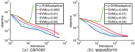
We first demonstrate the advantages of the adaptive learning rate scheme (in Section 2.2). Because of the lack of space, we only report results on breast cancer and waveform. Similar behavior is observed on the other data sets. For comparison, we also train the ρ-SVM using the multiplicative updating rule (with fixed η) in [Cristianini et al., 1999].
As can be seen from Figure 1, the performance of [Cristianini et al., 1999] is sensitive to the fixed choice of η. When η is small (e.g., η = 0.01 or smaller), the objective value decreases gradually. However, when η is slightly larger (say, at 0.02), the estimate will finally over-shoot (as indicated by the vertical lines) and convergence can no longer be obtained. On the other hand, our proposed adaptive scheme always converges much faster.
4.2 Accuracy and Speed
Next, we show that the proposed ensemble of partially trained hard-margin SVMs (Section 3.2) has comparable performance as the best-tuned soft-margin SVM (C-SVM). We use the Gaussian kernel k(xi, xj) = exp(-‖xi - xj‖2/β), with
9 astro-particles is downloaded from http://www.csie.ntu.edu.tw/∼cjlin/libsvmtools/datasets/, while others are from http://research.microsoft.com/users/jplatt/smo.html.
β = 1m ∑mi=1 ∥∥∥xi - 1m ∑mj=1 xj ∥∥∥2 . Each small data set in Table 1 comes with 100 realizations, and the performance is obtained by averaging over all these realizations. However, for each large data set, only one realization is available.
The ensemble is compared with the following:
- SVM (BEST): The best-performing SVM among all the C-SVMs obtained by the regularization path algorithm 10 [Hastie et al., 2005];
- SVM(LOO): TheC-SVMwhich has the best leave-oneout-error bound [Evgeniou et al., 2004] among those obtained by the regularization path algorithm;
- the Parzen window classifier, which is the first hypothesis added to the ensemble;
- the (hard-margin) ρ-SVM, which is the last hypothesis;
- the proposed ensemble.
All these are implemented in Matlab 11 and run on a 3.2GHz Pentium-4 machine with 1GB RAM.
| data set | SVM (BEST) | SVM (LOO) | Parzen window | ρ- SVM | proposed ensemble |
|---|---|---|---|---|---|
| cancer | 23.1 | 26.1 | 27.4 | 33.5 | 28.2 |
| diabetis | 24.8 | 28.9 | 33.4 | 34.5 | 24.8 |
| german | 22.6 | 24.9 | 29.8 | 29.3 | 23.7 |
| titanic | 22.7 | 25.5 | 23.3 | 45.2 | 22.5 |
| waveform | 11.2 | 18.8 | 22.0 | 11.2 | 10.0 |
| astro | 5.8 | 9.3 | 7.0 | 22.1 | 3.4 |
| adult1 | 16.3 | 17.7 | 24.1 | 19.4 | 15.9 |
| adult2 | 16.0 | 17.4 | 24.0 | 22.8 | 15.8 |
| adult3 | 16.1 | 16.2 | 24.1 | 19.7 | 15.9 |
| web1 | 2.3 | 2.8 | 3.0 | 14.4 | 2.8 |
| web2 | 2.1 | 2.2 | 3.0 | 3.4 | 2.1 |
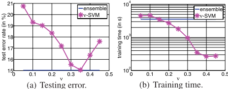
As can be seen from Table 2, the ensemble performs much better than the (hard-margin) ρ-SVM. Indeed, its accuracy is comparable to or sometimes even better that of SVM(BEST). Table 3 compares the time 12 for obtaining the ensemble with that of running the regularization path algorithm. As can be seen, obtaining the ensemble is much faster, and takes a small number of iterations. To illustrate the performance on large data sets, we experiment on the full adult data set in Table 1. The regularization path algorithm cannot be run on this large data. So, we use instead a ν-SVM (using LIBSVM 13 ) for comparison, where ν (unlike the C parameter in the C-SVM)
10 Alternatively, one can find the best-tuned SVM by performing a grid search on the soft-margin parameter. However, as each grid point then requires a complete re-training of the SVM, the regularization path algorithm is usually more efficient [Hastie et al., 2005].
11 The inner QP in the regularization path algorithm is solved by using the optimization package Mosek (http://www.mosek.com).
12 This includes the time for computing the kernel matrix, which can be expensive on large data sets. Moreover, time for computing the leave-one-out bound is not included in the timing of SVM(LOO).
13 Version 2.8.1 (C++ implementation) from http://www.csie.ntu.edu.tw/ cjlin/libsvm/.
| set | regularization path | proposed ensemble | |
|---|---|---|---|
| data | time | time | #iterations |
| cancer | 0.4 | 0.03 | 62.3 |
| diabetis | 3.1 | 0.1 | 65.5 |
| german | 22.2 | 0.3 | 44.9 |
| titanic | 0.08 | 0.08 | 434.4 |
| waveform | 2.7 | 0.1 | 42.4 |
| astro | 180.3 | 9.5 | 310 |
| adult1 | 243.3 | 10.7 | 42 |
| adult2 | 632.7 | 23.1 | 40 |
| adult3 | 957.3 | 49.1 | 104 |
| web1 | 2,853.7 | 64.3 | 33 |
| web2 | 6,978.7 | 129.9 | 125 |
can only be in [0, 1]. In the experiments, we further restrict ν to [0.05, 0.45] as the optimization becomes infeasible when ν falls outside this range. Moreover, low-rank approximation of the kernel matrix as mentioned in Section 3.3 is used.
As can be seen from Figure 2, training of the single besttuned ν-SVM takes 348.9s, while training the whole ensemble takes 3,555.1s, which is thus around 10 times slower. However, recall that ours is implemented in Matlab while LIBSVM is in C++. Moreover, as shown in Figure 2(b), SVM's training time is highly dependent on the value of ν. Hence, in practice, one has to perform SVM training together with ν parameter selection, which can be much more expensive than ensemble training.
5 Conclusion
In this paper, we show that the hard-margin SVM can be trained by a simple multiplicative updating rule. By casting its training as a Bregman projection problem, the optimal learning rate can be adaptively obtained from the data, and a finite convergence result can also be derived. Moreover, inspired from a connection between boosting and Bregman projection, we propose an ensemble classifier consisting of the partially trained hard-margin SVMs. Though its base hypothesis are hard-margin SVMs, experimental results show that this ensemble is resistant to overfitting and has comparable performance with the best-tuned soft-margin SVM. Moreover, training the whole ensemble (which in Matlab) is only 10 times slower than that of training the best-tuned SVM (in C++). Thus, we can obtain an accurate classifier while avoiding tedious tuning of the soft-margin parameter.
One problem with the ensemble is that its solution is no longer sparse. In the future, we will investigate the use of reducd set methods to alleviate this.
Acknowledgments
This research has been partially supported by the Research Grants Council of the Hong Kong Special Administrative Region.
@inproceedings{ijcai2007p176,
  title     = {Ensembles of Partially Trained SVMs with Multiplicative Updates},
  author    = {Tsang, Ivor W. and Kwok, James T.},
  booktitle = {Proceedings of the Twentieth International Joint Conference on
               Artificial Intelligence, {IJCAI-07}},
  publisher = {International Joint Conferences on Artificial Intelligence},
  editor    = {Manuela M. Veloso},
  pages     = {1089--1093},
  year      = {2007},
  url       = {https://ijcai.org/proceedings/2007/176},
}
TY - CPAPER TI - Ensembles of Partially Trained SVMs with Multiplicative Updates AU - Tsang, Ivor W. AU - Kwok, James T. T2 - Proceedings of the Twentieth International Joint Conference on Artificial Intelligence, IJCAI-07 PB - International Joint Conferences on Artificial Intelligence PY - 2007 SP - 1089 EP - 1093 UR - https://ijcai.org/proceedings/2007/176 ER -Copied
Machine-readable versions of this paper, for tools and AI agents:





