
A New Approach to Multiobjective A* Search
Proceedings of the Nineteenth International Joint Conference on Artificial Intelligence. Pages 218-222.
© 2005 International Joint Conferences on Artificial Intelligence
Abstract
The paper presents a new algorithm for multiobjective heuristic graph search problems. The algorithm presents some nice properties that are easily proven. Additionally, empirical tests show that substantial savings in memory can be achieved over previous proposals.
- [Bentley et al., 1978] J.L. Bentley, H.T. Kung, M. Schkol- nick, and C.D. Thomson. On the average number of max- ima in a set of vectors and applications. Journal of the ACM, 25(4):536-543, October 1978.
- [Dasgupta et al., 1999] Pallab Dasgupta, P.P. Chakrabarti, and S.C. DeSakar. Multiobjective Heuristic Search. Vieweg, Braunschweig/Wiesbaden, 1999.
- [Dechter and Pearl, 1985] Rina Dechter and Judea Pearl. Generalized best-first search strategies and the optimality of A*. Journal of the ACM, 32(3):505-536, July 1985.
- [Hart et al., 1968] P.E. Hart, N.J. Nilsson, and B. Raphael. A formal basis for the heuristic determination of minimum cost paths. IEEE Trans. Systems Science and Cybernetics SSC-4, 2:100-107, 1968.
- [Loui, 1983] Ronald P. Loui. Optimal paths in graphs with stochastic or multidimensional weights. Communications of the ACM, 26(9):670-676, September 1983.
- [Mandow and Pérez de la Cruz, 2003] L. Mandow and J.L. Pérez de la Cruz. Multicriteria heuristic search. European Journal of Operational Research, 150:253-280, 2003.
- [Pearl, 1984] Judea Pearl. Heuristics. Addison-Wesley, Reading, Massachusetts, 1984.
- [Perny and Spanjaard, 2002] Patrice Perny and Olivier Span- jaard. On preference-based search in state space graphs. In Proc. Eighteenth Nat. Conf. on AI, pages 751-756. AAAI Press, July 2002.
- [Stewart and White, 1991] Bradley S. Stewart and Chelsea C. White. Multiobjective A*. Journal of the ACM, 38(4):775-814, October 1991.
References were extracted automatically from the PDF and may contain errors.
Full text extracted automatically from the PDF; figures, tables and equations may differ. The PDF is the version of record.
1 Introduction
The multiobjective search problem is an extension of the shortest path problem where arc costs become vectors. This is a genuinely different problem since vector costs induce only a partial order relation.
Loui [1983] studied the extension of Dijkstra's algorithm to the multiobjective case, and showed that some stochastic search problems can be reduced to multiobjective ones. Stewart and White [1991] outlined MOA*, a multiobjective extension of A*, and presented proofs on admissibility, node expansion, and comparison of heuristics. Dasgupta et al. [1999] extended this work in several ways, including a version for non-monotone heuristics (MOA**), with applications in the area of VLSI design and the log cutting problem. Perny and Spanjaard [2002] presented a generalization of MOA* with application to a Web access problem. Mandow and P´erez de la Cruz [2003] presented a systematic extension of the heuristic search paradigm to the multicriteria case, and admissibility conditions for algorithms with different multicriteria preference relations (multiobjective, multiattribute, lexicographic, and goal-based).
This paper reconsiders the extension of A* to the multiobjective case and presents a new algorithm. The basic operations in A* are selection and expansion of open nodes at each iteration. In A* each open node stands for a single partial solution path that can be further expanded. However, as explained in the paper, this is no longer the case in multiobjective problems, where many interesting paths may reach the same node. The MOA* algorithm [Stewart and White, 1991], and subsequent extensions, were devised preserving node selection and expansion as the algorithm's basic operations. This paper presents an extension of A* to the multiobjective case that preserves path selection and expansion as the basic operations. Admissibility can be proven very easily. The new algorithm also shows important properties, analogous to those of A*, that are not shared by MOA*. Additionally, empirical tests show that the new algorithm offers substantial savings in memory over MOA*.
The paper is organized as follows. Section 2 reviews previous relevant work in scalar search and points out analogies and differences with the multiobjective search problem. Section 3 presents a new algorithm and illustrates its behaviour with a simple example. Relevant differences with MOA* are identified. Section 4 proves the admissibility of the new algorithm and a discusses on its efficiency. The performance results of multiobjective search over a set of randomly generated grid search problems is presented in section 5. Finally, conclusions and future research are briefly summarized.
2 Scalar and multiobjective search
2.1 Previous results in scalar graph search
The shortest path problem can be stated as follows: given a locally finite labelled directed graph G = (N,A, c), of |N| nodes, and |A| arcs (n, n′ ) labelled with positive costs c(n, n′ ) ∈ R, a start node s ∈ N, and a set of goal nodes Γ ⊆ N, find the minimum cost path in G from s to a node in Γ.
The A* algorithm [Hart et al., 1968] is an efficient solution to this problem. It is a best-first search algorithm that uses a search tree to store the set of known interesting partial solution paths, a list of open nodes that can be further expanded, and a characteristic evaluation function f(n) = g(n) + h(n) to select the next open node to be expanded. While function g(n) denotes the known cost of the path stored in the tree from s to n, the heuristic function h(n) estimates of the cost of a solution from node n to a goal node. Heuristic functions can be devised for particular problems depending on their semantics.
Beautiful results have been presented to analyse the relation between the accuracy of h(n) and the properties of A*. Admissibility: Let h∗ (n) be the real optimal cost of a path from n to a goal node. When the heuristic is an optimistic estimate (h(n) ≤ h∗ (n) ∀n), the search is admissible, i.e. if a solution exists it is guaranteed to find an optimal one. With additional constraints (h(n) ≥ 0 ∀n, and c(n, n′ ) ≥ ϵ > 0 ∀(n, n′ ) ∈ A) A* is admissible even on infinite graphs.
Efficiency: When ∀n h(n) = 0, A* behaves like Dijkstra's algorithm. When h(n) is consistent or satisfies the equivalent monotone property,
A* solves the problem in O(|N|) iterations, storing O(|N|) nodes in memory, in the worst case. Particularly, if c∗ denotes the optimal solution cost, A* will always expand all nodes with f(n) < c∗ , but at most those with f(n) ≤ c∗ . Therefore, given an optimistic estimate, big values of h(n) can push the evaluation of more and more nodes beyond the f(n) = c∗ frontier, reducing search effort.
Optimality: When the heuristic is monotone A* can also be proven optimal among the class of admissible best-first algorithms that are guided by path-dependent evaluation functions [Dechter and Pearl, 1985].
2.2 Extension to the multiobjective case
The multiobjective search problem can be stated as follows: given a locally finite labelled directed graph G = (N, A,⃗c), of |N| nodes, and |A| arcs (n, n′ ) labelled with positive vectors ⃗c(n, n′ ) ∈ Rq , a start node s ∈ N, and a set of goal nodes Γ ⊆ N, find the set of non-dominated cost paths in G from s to nodes in Γ.
In multiobjective problems cost vectors ⃗c(n, n′ ) induce only a partial order preference relation ≺ called dominance,
where fi denotes the i-th element of vector ⃗ f .
Therefore, given two q-dimensional vectors ⃗ f and ⃗ f ′ , it is not always possible to rank one as better than the other. For example, in a two dimensional cost space, vector (2, 3) dominates (2, 4), but no dominance relation exists between vectors (2, 3) and (3, 2).
The essence of the multiobjective search problem is to find the set of all non-dominated solution paths. Therefore, an analogy could be traced to a version of A* that aims at finding all optimal paths. However, some important differences with the scalar search problem can be pointed out.
First of all, given the dominance preference relation, two (or more) uncomparable (non-dominated) paths may reach any given node from the same or different parents. Several important consequences can be identified:
- The search tree used byA* to record the best known path to generated nodes is no longer sufficient. A directed acyclic graph can be used instead, to record the set of non-dominated known paths to generated nodes.
- The number of generated nodes may no longer be a realistic estimate of the memory needed by the algorithm. All arcs and non-dominated cost vectors reaching each node need to be recorded as well. Let M be an upper bound on the size of the largest set of nondominated vectors in a node, and O(M) a bound on the size of the approximations to these sets. In the worst case O(MN) cost vectors need to be stored. Bentley et al. [1978] prove that the average number of nondominated q-dimensional vectors in a set of size L is O((log|L|)q-1 ), provided all (n!)q relative orderings are equally probable.
- Finally, each time a new path is generated to a known node, its cost may need to be tested for dominance with the set of all known costs reaching the node.
In general, heuristic estimates will involve a set of vectors H(n) for each node n, estimating cost vectors of paths from n to each goal node. Therefore, for each path Psn from s to n with cost ⃗gP , there will be a set of heuristic evaluation vectors, F (Psn). This function is the multiobjective analogue to f(n) in A*,
where nondom(X) denotes the set of non-dominated vectors in set X.
Finally, note that at each iteration, A* selects and expands an open node, i.e. considers all the possible extensions of the path stored in the search tree to that node. In A* each open node stands for a single partial solution path that can be further expanded. However, in the multiobjective case, if an acyclic graph is used instead of a tree to record partial solutions, this will no longer be the case. The MOA* algorithm [Stewart and White, 1991] was devised preserving node selection and expansion as the algorithm's basic operations. The next section introduces an extension of A* to the multiobjective case that preserves path selection and expansion as the basic operations.
3 A new algorithm for multiobjective A* search
3.1 Brief description
The pseudocode of a new multiobjective A* search algorithm is shown in table 1.
In accordance to the considerations in sec 2.2, we will devise our extension of A* to the multiobjective case in the following way:
- The algorithm uses an acyclic search graph SG to record interesting partial solution paths. For each node n in SG two sets, Gcl(n) and Gop(n), denote the sets of nondominated cost vectors of paths reaching n that have or have not been explored yet respectively (i.e. closed or open). Each cost vector in this sets labels one or more pointers emanating from n to its parents with that cost. Initially, s is the only node in SG.
- The algorithm keeps a list OPEN, of partial solution paths that can be further expanded. For each node n in SG and each nondominated cost vector ⃗g ∈ Gop(n), there will be a corresponding triple (n,⃗g, F(n,⃗g)) in OPEN. Initially, (s,⃗gs, F(s,⃗gs)) is the only triple in OP EN .
- At each iteration, the algorithm will consider the extension of an open triple (n,⃗g, F) that stands for a partial solution path from s to n with cost ⃗g.
- Two sets, GOALN and COSTS, record all goal nodes reached and all non-dominated cost vectors to goal nodes respectively. Once a solution is known its cost vector can be used to discard (filter) dominated open triples.
- Search terminates only when the OPEN list is empty, i.e. when all open triples have been selected or filtered.
3.2 Example
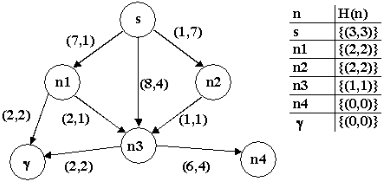
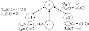
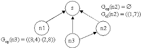
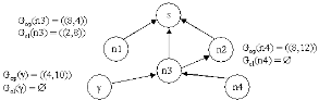
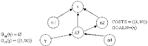
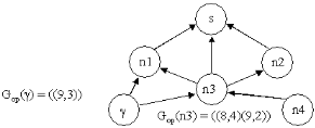
We will illustrate the workings of the previous algorithm on the sample graph in figure 1. A heuristic evaluation function H(n) is also presented. A single heuristic vector is given for each node for the sake of simplicity. A trace of the search graph is shown in figures 2-6. Values of Gop and Gcl are shown at each iteration. Values that do not change from the previous iteration are omitted for brevity. Table 2 shows a trace of OPEN.
At iteration 1, SG has only node s at its root, Gop(s) = {(0, 0)}, and Gcl(s) = ∅. The only path in OPEN is selected, and its three extensions to nodes n1, n2, and n3 added to SG and OPEN. At iteration 2 two alternatives have nondominated estimates in OPEN (n1 with estimate (9, 3), and n2 with estimate (3, 9)). Let's assume ties between nondominated estimates are always broken choosing the smaller first component in estimated cost vectors. The path leading to n2 would be selected, and its extension to n3 generated. At iteration 3 two non-dominated paths lead to node n3 (each cost vector in Gop(n3) would label a different pointer). One of them is non-dominated in OPEN and selected. At iteration 4 a path leading to the goal node γ has a non-dominated estimate inOPEN. It is selected, added toGOALN, and its cost vector included in COSTS. At iteration 5 the path leading to node n4 has been filtered (its estimate is dominated by the vector in COSTS). The only non-dominated alternatives are selected at iterations 5 and 6. At iteration 6 a new solution path leading to γ is selected. Therefore, the set COSTS is updated to {(4, 10)(9, 3)}. At iteration 7 all remaining alternatives are filtered and OPEN is empty. The algorithm would backtrack from γ returning the two paths found with costs (4, 8) and (9, 3).
Table 1: A new path expansion algorithm for multiobjective A* search.
- CREATE:
- An acyclic search graph SG rooted in s.
- List of alternatives, OPEN = {(s, ⃗gs, F(s, ⃗gs)) }.
- Two empty sets, GOALN, COSTS.
- CHECK TERMINATION. If OPEN is empty, then backtrack in SG from the nodes in GOALN and return the set of solution paths with costs in COSTS.
- PATH SELECTION. Select an alternative (n,⃗gn, F) fromOPENwith ⃗ f ∈ F non-dominated in OPEN, i.e.
Delete (n,⃗gn, F) from OPEN, and move ⃗gn from Gop(n) to Gcl(n).
- SOLUTION RECORDING. If n ∈ Γ, then
- Include n in GOALN and ⃗gn in COSTS.
- Eliminate from OPEN all alternatives (x, gx, Fx) such that all vectors in Fx are dominated by ⃗gn (FILTERING).
- Go back to step 2
- PATH EXPANSION: If n ̸∈ Γ, then For all successors nodes m of n that do not produce cy-
cles in SG do:
- (a) Calculate the cost of the new path found to m: ⃗gm = ⃗gn + ⃗c(n, m).
- (b) If m is a new node
- Calculate Fm = F(m,⃗gm) filtering estimates dominated by COSTS.
- If Fm is not empty, put (m,⃗gm, Fm) in OPEN, and put ⃗gm in Gop(m) labelling a pointer to n.
- Go to step 2.
else (m is not a new node), in case
- ⃗gm ∈ Gop(m) or ⃗gm ∈ Gcl(m): label with ⃗gm a pointer to n, and go to step 2.
- If ⃗gm is non-dominated by any cost vectors in Gop(m) ∪ Gcl(m) (a path to m with new cost has been found), then :
- Eliminate from Gop(m) and Gcl(m) vectors dominated by ⃗gm
- Calculate Fm = F(m,⃗gm) filtering estimates dominated by COSTS.
- If Fm is not empty, put (m,⃗gm, Fm) in OPEN, and put ⃗gm in Gop(m) labelling a pointer to n.
- Go to step 2.
- Otherwise: go to step 2.
| It. | OPEN |
| 1 | (s, (0, 0), ((3, 3))) ← |
| 2 | (n1, (7, 1), ((9, 3))) (n2, (1, 7), ((3, 9))) ← (n3, (8, 4), ((9, 5))) dom |
| 3 | (n1, (7, 1), ((9, 3))) (n3, (8, 4), ((9, 5))) dom (n3, (2, 8), ((3, 9))) ← |
| 4 | (n1, (7, 1), ((9, 3))) (n3, (8, 4), ((9, 5))) dom (n4, (8, 12), ((8, 12))) dom (γ, (4, 10), ((4, 10))) ← |
| 5 | (n1, (7, 1), ((9, 3))) ← (n3, (8, 4), ((9, 5))) dom |
| 6 | (n3, (8, 4), ((9, 5))) dom (γ, (9, 3), ((9, 3))) ← (n3, (9, 2), ((10, 3))) dom |
3.3 Selection and expansion: paths versus nodes
MOA* has been for more than a decade the reference multiobjective heuristic search algorithm. Unlike the algorithm presented in section 3.1, MOA* is built around the idea of node selection and expansion. Particularly, it makes no distinction in SG between the sets Gop(n) and Gcl(n), and a single set G(n) = Gop(n) ∪ Gcl(n) is kept for each node. A heuristic evaluation function F(n) is defined for each node,
F (n) = nondom{ ⃗ f | ⃗ f = ⃗g+⃗h ∧⃗g ∈ G(n)∧⃗h ∈ H(n)} The OPEN list can be considered a list of pairs (n, F(n)) where nodes with non-dominated ⃗ f ∈ F(n) are selected. The distinction between individual paths reaching each node n is lost and, accordingly, all known paths reaching each node n are either simultaneously open or closed. Essentially MOA* presents two distinguishing features when compared to the algorithm in section 3.1:
- Each time a newnon-dominated path is found to a closed node, the whole node is put back into OPEN.
- Each time a node is selected for expansion, all known non-dominated paths reaching that node are extended.
The first difference may result in unnecesary reexpansion of nodes. The second may result in unnecessary extension of paths in SG and storage of uninteresting cost vectors. Additionally, when a goal node γ is selected, all cost vectors in G(γ) may enter in COSTS. In general, it is not possible to know which of these cost vectors belong to truly nondominated solutions until all of them have been found.
These differences can be illustrated with the example presented in section 3.2. Provided ties in the selection of OPEN paths were broken in the same way, search with MOA* would produce the same results in the first two iterations. In iteration 3, the selection of node n3 for expansion would produce in MOA* the extension of both known nondominated paths to that node. Accordingly, all cost vectors in G(n3) = {(8, 4)(2, 8)} would be extended resulting in G(n4) = {(14, 8)(8, 12)} and G(γ) = {(10, 6)(4, 10)}, and node n3 would be marked as closed. Note that the new algorithm did not need to store cost vectors (14, 8) in node n4, or (10, 6) in γ.
At iteration 4 node γ would be selected, and two different cost vectors {(10, 6)(4, 10)} would be included in COSTS. One of them does not belong to a truly non-dominated solution, but MOA* will not be able to tell until termination.
Finally, note that at iteration 5, the expansion of node n1 results in a new non-dominated path to n3. MOA* would place accordingly n3 back in OPEN with all its heuristic evaluation cost vectors. This implies that prior to termination, MOA* will need to reexpand n3. This was unnecessary in the new algorithm since the newly found path to n3 can never lead to a non-dominated solution.
4 Properties
This section presents proofs on the admissibility of the new algorithm presented in section 3, and bounds on the number of paths selected and stored in memory.
A scalar algorithm is said to be admissible if it is guaranteed to return an optimal solution whenever a solution exists.
We extend the definition as follows: a multiobjective search algorithm is N-admissible if it terminates with the set of all non-dominated solutions whenever this set is finite and nonempty, or if it does not terminate whenever this set is infinite.
Let C∗ be the set of non-dominated solution costs, ⃗g(P) the cost vector of path P, and ⪯ the relation "dominates or equals". Let ⃗m∗ = (m∗1 ,m∗2 , . . .m∗q ) denote the ideal optimal cost vector, i.e. a vector that would attain the optimal cost for each individual dimension. Note that problems where ideal optimal solutions are reachable are highly unusual.
The proofs presented in this section rely on a set of reasonable assumptions, analogous to those presented in [Stewart and White, 1991] to prove the admissibility of MOA*:
- The graph G = (N, A) to be searched is locally finite.
- The heuristic function H(n) is admissible, i.e. for all non-dominated solution paths P ∗ = (s, n1, . . . , ni, ni+1 . . . γk), γk ∈ Γ and each subpath P ∗
- i = (s, n1, . . . , ni) of P ∗ , ∃⃗h ∈ H(ni) | ⃗g(P ∗ i ) +⃗h ⪯ ⃗g(P ∗ )
- For infinite graphs,
- (a) hk ≥ 0 ∀k ∀n ∀⃗h ∈ H(n)
- (b) ⃗ck(n, n′ ) ≥ ϵ > 0 ∀k ∀(n, n′ ) ∈ A
Theorem 1 : For each non-dominated solution path P ∗ = (s, n1, . . . , ni, ni+1 . . . γ) with cost ⃗g(P ∗ ) = ⃗c∗ , there is always before its discovery a subpath P ∗ i = (s, n1, . . . , ni) of P ∗ such that: a)P ∗ i is recorded in SG; b) ⃗g(P ∗ i ) ∈ Gop(ni); c) ∃⃗ f ∈ F(P ∗ i ) | ⃗ f ⪯ ⃗c∗ .
Proof. We first consider parts (a), and (b). The proposition is true at iteration 1, when s is in OPEN and at the root of SG. It is also true in subsequent iterations, since subpaths of non-dominated solutions can never be pruned from SG. Let P ∗ i make the proposition true for some non-dominated solution P ∗ . By definition, P ∗ i is non-dominated to ni, therefore ⃗g(P ∗ i ) will never be removed from Gop(ni) unless (ni, ⃗g(P ∗ i ), F(P ∗ i )) is selected for expansion. Upon selection, if ni = γ, then P ∗ i = P ∗ is discovered. If ni ̸= γ, a new non-dominated path to ni+1, P ∗ i+1 = (s, n1, . . . , ni, ni+1) will be generated, ⃗g(P ∗ i+1 ) included in Gop(ni+1) and P ∗ i+1 will satisfy the proposition. Part (c) follows then trivially from the definition of F and admissible heuristic. This, in turn, prevents P ∗ or any of its subpaths from filtering.
Theorem 2 If there is a solution, the algorithm terminates even on infinite graphs.
Proof. All best first search algorithms that prune cycles terminate on finite graphs [Pearl, 1984]. Given the assumptions for infinite graphs, all paths P with length longer than
will trivially attain ⃗g(P) such that ⃗c∗ ≺ ⃗ f for all ⃗c∗ ∈ C∗ and all ⃗ f ∈ F(P). Since the graph G is locally finite, there can only be a finite number of partial solution paths non-dominated by C∗ . Therefore, from theorem 1, all nondominated solutions will eventually be found, and all infinite paths will be pruned or filtered from OPEN in a finite number of steps.
Theorem 3 The algorithm is N-admissible.
Proof. From theorems 1 and 2 follows that the algorithmwill always terminate with all non-dominated solutions. It suffices to show that a dominated solution can never be selected. Let's assume, for the purpose of contradiction, that a dominated solution P with cost ⃗gP is selected, i.e. exists ⃗c∗ ∈ C∗ with ⃗c∗ ≺ ⃗gP , and F(P) = {⃗gP}. It must be ⃗c∗ ̸∈ COSTS, for otherwise P would have been filtered. Now, from theorem 1, for all ⃗c∗ ∈ C∗ not found yet there is at least one path Pi = (s, . . . , ni) such that exists ⃗ f ∈ F(Pi)) with ⃗ f ⪯ ⃗c∗ , and (ni,⃗g(Pi), F(Pi)) is in OPEN. Now, from the transitivity of the dominance relation follows that ⃗ f ⪯ ⃗c∗ ≺ ⃗gP and P cannot be selected for expansion.
Corolary 1 At any time COSTS ⊆ C∗ . Therefore, the algorithm may terminate at any time returning the set of nondominated solutions found so far.
Corolary 2 All paths P in SG with ⃗ f ∈ F(P) such that ∀⃗c∗ ∈ C∗ ,⃗c∗ ⊀ ⃗ f will either be pruned at later iterations, or selected for expansion.
Corolary 3 No path P such that ∀⃗ f ∈ F(P) ∃⃗c∗ ∈ C∗ ,⃗c∗ ≺ ⃗ f will ever be selected for expansion.
Corolary 4 For each path P recorded in SG such that ∀⃗ f ∈ F(P) ∃⃗c∗ ∈ C∗ ,⃗c∗ ≺ ⃗ f, its extensions will never be recorded in SG.
Proofs of corolaries 1, 3 and 4 are trivial from the proof of theorem 3. Corolary 2 is also trivial since otherwise the algorithmwould not terminate.
Note that a version of A* that found all optimal paths would also satisfy corolary 1. Corolaries 2 and 3 give lower and upper bounds on the paths selected for expansion. These are analogous to the efficiency bounds of A* (see section 2.1).
The example presented in section 3.2 shows that corolaries 1, 3, and 4 do not apply to MOA*. Particularly, for MOA*, no upper bound can be given for the cost of paths whose extensions will be recorded in SG depending on C∗ .
5 Experimental test
5.1 Search space and practical issues
Search in square grids of nodes was used to test the algorithms. These experiments provide further insight into the workings of both algorithms, as well as a preliminary evaluation of the memory savings that can be achieved with the new algorithm. In two dimensional grids, each node (identified by its coordinates) has its four neighbours as successors. Note that, for this problem, storing each node takes less space than storing each cost vector for q > 2.
Vector costs were generated randomly with integer components in the range [1, 10]. A single goal node was generated for each problem instance, at a random distance between 2 and 30 arcs from the start node. Manhattan distance to the goal can be used as an optimistic cost estimate for each component of the cost vectors.
A lexicographic order was used to sort alternatives in the OPEN set, as sugested in [Loui, 1983]. Particularly, only the current lexicographically optimal evaluation vector ⃗ f is placed in OPEN for each node with open alternatives. Therefore, the size of OPEN is O(|N|) in the worst case for both algorithms, and alternatives can be deleted and inserted in O(log|N|) in a binary heap. Proofs on admissibility are not affected by this selection mechanism, since a lexicographic optimum is always a non-dominated vector.
5.2 Results
Table 3 summarizes relevant parameters of the search carried out over a set of 1000 problems by both algorithms 1 . The set involved two-dimensional grids with three objectives. The number of nodes involved in selections was the same on both cases. The new algorithm performed 1208% more iterations, but took only 3% more time on average to complete the searches. In fact the new algorithm performed slower than MOA* only in 297 of the searches and faster in 669 of them. On the memory side, the number of nodes stored by the new algorithm was slightly higher, the number of arcs slightly lower, and the number of stored cost vectors was clearly lower. MOA* had lower requirements only in two problem instances, and needed 41.4% more space on average.
Several phenomena can be observed. The higher average size of the OPEN list may slow insertions and deletions in the new algorithm. An average search with MOA* needed to expand only 2.47 goal nodes to find all solution paths, while the new algorithm needed 75.57 on average (at least one for each cost vector in C∗ ). This suggests MOA* may benefit in some cases from earlier filtering, accounting for the slightly lower number of nodes recorded in SG and the two very simple cases in which MOA* stored less cost vectos. However, memory consumption is clearly dominated by the number of paths (or cost vectors) stored in SG where the new algorithm performs consistently better.
In summary, the new algorithm performed much better in memory requirements but found solutions slightly more slowly on average. Time values are the only measure subject to implementation details and should be taken with caution, but show clearly that the number of iterations is not a good indicator to compare the running time of both algorithms.
6 Conclusions and future work
A new admissible algorithm based on path selection and expansion has been presented for multiobjective heuristic search. The algorithm is amenable to formal analysis and presents several interesting properties: the algorithm may be stopped at any time, returning the subset of non-dominated solutions found so far; bounds can be given on the number of paths stored in SG, and selected for expansion, as a function of C∗ . An example is shown where MOA*, a previous algorithm, violates the upper bounds. Preliminary experimental tests confirm that the new algorithm consistently saves substantial amounts of memory, though more complete experimental evaluation in needed.
The properties presented in the paper are a necessary first step in a proper analysis on the influence of monotonicity and
1 Problem sets and solutions are available from the authors.
| New algorithm Iterations Goal nodes sel. Nodes in SG Arcs in SG Cost vect. in SG Avg. OPEN size Time (s) MOA* Iterations Goal nodes sel. Nodes in SG Arcs in SG Cost vect. in SG Avg. OPEN size Time (s) | 8396.22 ( 6.00 ; 63722.00 ; 10024.38) 75.57 ( 1.00 ; 433.00 ; 77.26) 427.60 ( 9.00 ; 1147.00 ; 245.25) 805.30 ( 9.00 ; 2318.00 ; 498.22) 9248.19 ( 9.00 ; 67904.00 ; 10809.98) 171.89 ( 1.67 ; 524.04 ; 112.76) 7.99 ( 0.00 ; 169.18 ; 16.35) 694.80 ( 6.00 ; 2338.00 ; 458.23) 2.47 ( 1.00 ; 15.00 ; 1.84) 411.11 ( 9.00 ; 1124.00 ; 237.66) 817.34 ( 9.00 ; 2401.00 ; 504.26) 13080.49 ( 9.00 ; 88684.00 ; 14648.51) 40.56 ( 1.67 ; 80.71 ; 16.25) 7.75 ( 0.00 ; 149.86 ; 13.66) |
heuristic accuracy in the performance of the algorithm. Future work includes detailed average time complexity analysis of the algorithms, a detailed study on the influence of heuristic information on time and space efficiency, and, eventually, an extension of Dechter and Pearl's [1985] analysis on the optimality of A* to the multiobjective case.
@inproceedings{ijcai2005p96,
  title     = {A New Approach to Multiobjective A* Search},
  author    = {Mandow, Lawrence and Pérez-de-la-Cruz, José-Luis},
  booktitle = {Proceedings of the Nineteenth International Joint Conference on
               Artificial Intelligence, {IJCAI-05}},
  publisher = {International Joint Conferences on Artificial Intelligence},
  editor    = {Leslie Pack Kaelbling and Alessandro Saffiotti},
  pages     = {218--222},
  year      = {2005},
  url       = {https://ijcai.org/proceedings/2005/96},
}
TY - CPAPER TI - A New Approach to Multiobjective A* Search AU - Mandow, Lawrence AU - Pérez-de-la-Cruz, José-Luis T2 - Proceedings of the Nineteenth International Joint Conference on Artificial Intelligence, IJCAI-05 PB - International Joint Conferences on Artificial Intelligence PY - 2005 SP - 218 EP - 222 UR - https://ijcai.org/proceedings/2005/96 ER -Copied
Machine-readable versions of this paper, for tools and AI agents:





