
Sensitivity Analysis in Markov Networks
Proceedings of the Nineteenth International Joint Conference on Artificial Intelligence. Pages 1300-1304.
© 2005 International Joint Conferences on Artificial Intelligence
Abstract
This paper explores the topic of sensitivity analysis in Markov networks, by tackling questions similar to those arising in the context of Bayesian networks: the tuning of parameters to satisfy query constraints, and the bounding of query changes when perturbing network parameters. Even though the distribution induced by a Markov network corresponds to ratios of multi-linear functions, whereas the distribution induced by a Bayesian network corresponds to multi-linear functions, the results we obtain for Markov networks are as effective computationally as those obtained for Bayesian networks. This similarity is due to the fact that conditional probabilities have the same functional form in both Bayesian and Markov networks, which turns out to be the more influential factor. The major difference we found, however, is in how changes in parameter values should be quantified, as such parameters are interpreted differently in Bayesian networks and Markov networks.
- [Castillo et al., 1997] Enrique Castillo, José Manuel Gutiérrez, and Ali S. Hadi. Sensitivity analysis in discrete Bayesian networks. IEEE Transactions on Systems, Man, and Cybernetics, Part A (Systems and Humans), 27:412-423, 1997.
- [Chan and Darwiche, 2002] Hei Chan and Adnan Darwiche. When do numbers really matter? Journal of Artificial In- telligence Research, 17:265-287, 2002.
- [Chan and Darwiche, 2004] Hei Chan and Adnan Darwiche. Sensitivity analysis in Bayesian networks: From single to multiple parameters. In Proceedings of the Twentieth Conference on Uncertainty in Artificial Intelligence (UAI), pages 67-75, Arlington, Virginia, 2004. AUAI Press.
- [Chan and Darwiche, 2005] Hei Chan and Adnan Darwiche. A distance measure for bounding probabilistic belief change. International Journal of Approximate Reasoning, 38:149-174, 2005.
- [Darwiche, 2003] Adnan Darwiche. A differential approach to inference in Bayesian networks. Journal of the ACM, 50:280-305, 2003.
- [Geman and Geman, 1984] Stuart Geman and Donald Ge- man. Stochastic relaxation, Gibbs distributions, and the Bayesian restoration of images. IEEE Transactions in Pat- tern Analysis and Machine Intelligence, 6:721-741, 1984.
- [Jensen, 1999] Finn V. Jensen. Gradient descent training of Bayesian networks. In Proceedings of the Fifth European Conference on Symbolic and Quantitative Approaches to Reasoning with Uncertainty (ECSQARU), pages 190-200, Berlin, Germany, 1999. Springer-Verlag.
- [Jensen, 2001] Finn V. Jensen. Bayesian Networks and De- cision Graphs. Springer-Verlag, New York, 2001.
- [Kjærulff and van der Gaag, 2000] Uffe Kjærulff and Linda C. van der Gaag. Making sensitivity analysis computationally efficient. In Proceedings of the Sixteenth Conference on Uncertainty in Artificial Intelligence (UAI), pages 317-325, San Francisco, California, 2000.
- [Laskey, 1995] Kathryn B. Laskey. Sensitivity analysis for probability assessments in Bayesian networks. IEEE Transactions on Systems, Man, and Cybernetics, 25:901- 909, 1995.
- [Pearl, 1988] Judea Pearl. Probabilistic Reasoning in Intel- ligent Systems: Networks of Plausible Inference. Morgan Kaufmann Publishers, San Francisco, California, 1988.
References were extracted automatically from the PDF and may contain errors.
Full text extracted automatically from the PDF; figures, tables and equations may differ. The PDF is the version of record.
1 Introduction
In the domain of uncertainty reasoning, graphical models are used to embed and represent probabilistic dependencies between random variables. There are two major types of graphical models: Bayesian networks [Pearl, 1988; Jensen, 2001] and Markov networks [Pearl, 1988]. In both models, there are two components, a qualitative part and a quantitative part. In the qualitative part, a graph is used to represent the interactions between variables, such that variables with direct interactions are connected by edges, and information of independence relationships between variables can be inferred from the network structure. In the quantitative part, a set of parameters are specified to quantify the strengths of influences between related variables. The joint probability distribution can then be induced from the two components.
Bayesian networks and Markov networks differ in both the qualitative and quantitative parts of the models. For the qualitative part, directed edges are used in a Bayesian network to represent influences from one variable to another, and no cycles are allowed in the graph, while undirected edges are used in a Markov network to represent symmetrical probabilistic dependencies between variables.
For the quantitative part, the parameters in a Bayesian network are specified in conditional probability tables (CPTs) of the variables, where each CPT consists of the conditional probability distributions of a variable given instantiations of its parents, which are the variables that directly influence this variable. Because these parameters are conditional probabilities, they are more intuitive, but have to obey certain properties. For example, the probabilities in each conditional distribution must be normalized and sum to 1. On the other hand, the parameters in a Markov network are given in potentials, defined over instantiations of cliques, which are maximal sets of variables such that every pair of variables in a clique are connected by an edge. These parameters do not need to be normalized and can be changed more freely.
The topic of sensitivity analysis is concerned with understanding and characterizing the relationship between the local parameters quantifying a network and the global queries computed based on the network. Sensitivity analysis has been investigated quite comprehensively in Bayesian networks [Laskey, 1995; Castillo et al., 1997; Jensen, 1999; Kjærulff and van der Gaag, 2000; Chan and Darwiche, 2002; 2004; 2005]. Earlier work on the subject has observed that the distribution induced by a Bayesian network corresponds to multi-linear functions, providing effective computational methods for computing ∂Pr(e)/∂θx|u: the partial derivative of a joint probability with respect to a network parameter. These earlier results were recently pursued further, providing effective methods for solving the following problems:
- What is the necessary parameter change we need to apply such that a given query constraint is satisfied? For example, we may want some query value Pr(z | e) to be at least p by changing network parameters. Efficient solutions were given to this problem for computing minimum changes for single parameters [Chan and Darwiche, 2002], and multiple parameters in a single CPT [Chan and Darwiche, 2004].
- What is the bound on the change in some query value if we apply an arbitrary parameter change? Here, we are interested in finding a general bound for any query and any parameter of any network. It has been shown that the log-odds change in any conditional query in a
Bayesian network is bounded by the log-odds change in any single parameter [Chan and Darwiche, 2002].
- What is the bound on the difference between some query value induced by two networks that have the same structure but different parameter values? The solution to this problem is based on a newly proposed distance measure [Chan and Darwiche, 2005], which allows one to bound the difference between the query values under two distributions. Based on this distance measure, and given two Bayesian networks that differ by only a single CPT, the global distance measure between the distributions induced by the networks can be computed from the local distance measure between the CPTs, thereby allowing one to provide a bound on the difference between the query values. Moreover, if we are given multiple CPTs that do not intersect with each other, the global distance measure can still be computed as the sum of the local distance measures between the individual CPTs.
In this paper, we address these key questions of sensitivity analysis but with respect to Markov networks. The main question of interest is the extent to which these promising results hold in Markov networks as well. There is indeed a key difference between Bayesian networks and Markov networks which appears to suggest a lack of parallels in this case: whereas the joint distribution induced by a Bayesian network corresponds to multi-linear functions, the joint distribution induced by a Markov network corresponds to ratios of multi-linear functions. As it turns out, however, the conditional probability function has the same functional form in both Bayesian and Markov networks, as ratios of multi-linear functions. This similarity turns out to be the key factor here, allowing us to derive similarly effective results for Markov networks. This is greatly beneficial because we can answer the previous three questions in the context of Markov networks as well, with the same computational complexity. For example, we can go through each parameter in a Markov network, compute the minimum single parameter changes necessary to enforce a query constraint, and find the one that perturbs the network the least. Alternatively, we can change all parameters in a single clique table, and find the change that minimizes network perturbation. Afterwards, we can compute a bound on any query change using the distance measure incurred by the parameter change.
Our results, however, point to a main semantical difference between Bayesian networks and Markov networks, relating to how one should quantify and measure parameter changes. That is, how should one quantify a parameter change from .3 to .4? In a Bayesian network, parameters are interpreted as conditional probabilities, and the measure which quantifies the change is the relative odds change in the parameter value. This means query values are much more sensitive to changes in extreme probability values, whether close to 0 or 1. On the other hand, in a Markov network, parameters are interpreted as compatibility ratios, and the measure which quantifies the change is the relative change in the parameter value. This difference stems from how the parameters in the two models are interpreted and will be explained in more depth later.
This paper is structured as follows. Section 2 is dedicated to the definition and parameterization of Markov networks. Section 3 presents a procedure which tunes parameters in a Markov network in order to satisfy a query constraint. Section 4 introduces a distance measure that can be used to bound query change between distributions induced by two Markov networks. Section 5 concludes the paper.
2 Markov networks
A Markov network M = (G,Θ) consists of two parts: the network structure in terms of an undirected graph G, and the parameterization Θ. Each node in the undirected graph G represents a random variable, and two variables are connected by an edge if there exists a direct interaction between them. The absence of an edge between two variables means any potential interaction between them is indirect and conditional upon other variables.
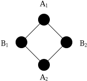
As an example, consider four individuals, A1,A2,B1,B2, and we wish to represent the possible transmission of a contagious disease among them. A network structure which consists of these variables is shown in Figure 1. Each pair of variables {Ai, Bj} is connected by an edge, meaning these pairs of individuals are in direct contact of each other. However, A1 and A2 are not connected with an edge, meaning they do not interact directly with each other, although diseases can still be transmitted between them indirectly through B1 or B2.
To quantify the edges in a Markov network, we first define cliques in the network structure. A clique C is a maximal set of variables where each pair of variables in the set C is connected by an edge. In the network structure in Figure 1, there are four cliques: {A1,B1}, {A1,B2}, {A2,B1}, {A2,B2}.
For each clique C, we define a table ΘC that assigns a nonnegative number θc to each instantiation c of variables C, which measures the relative degree of compatibility associated with each instantiation c. The numbers given indicate the level of compatibility between the values of the variables in the clique, where direct interactions exist between every pair of variables. For example, in our example network, we define the same clique table ΘAi,Bj shown in Table 1 for each clique {Ai, Bj}. For example, it can be viewed that both Ai and Bj not having the disease is four times more compatible than both Ai and Bj having the disease, since θ ¯ ai, ¯ bj = 4θai,bj . 1
1 Parameters may be estimated on an ad hoc basis [Geman and Geman, 1984] or by statistical models. It can be difficult to assign meanings and numbers to Markov network parameters intuitively [Pearl, 1988, pages 107-108].
| Ai | Bj ΘAi,Bj |
| ai | bj 1 |
| ai | ¯ bj 2 |
| ¯ ai | bj 3 |
| ¯ ai | ¯ bj 4 |
2.1 Joint and conditional probabilities induced by Markov networks
We now proceed to find the distribution induced by a Markov network. If X is the set of all variables in the Markov network M = (G,Θ), the joint potential ψ over X induced by M is defined as:
That is, ψ(x) is the product of parameters θc in each clique C, such that instantiation c is consistent with x. The joint distribution P rM induced by Markov network M is then defined as its normalized joint potential:
where K = 1/ ∑x ψ(x) is the normalizing constant. From this equation, we can easily verify that the specific parameter values in a clique are not important, but their ratios are. This is a major departure from Bayesian networks, where specific parameter values in CPTs are important.
Given the network structure in Figure 1 with the parameterization in Table 1, we can compute the joint probability of any full instantiation of variables induced by our example network. For example, the joint probability of a1, ¯ a2, b1, ¯ b2 is equal toKθa1,b1 θa1, ¯ b2 θ ¯ a2,b1 θ ¯ a2, ¯ b2 = K · 1 · 2 · 3 · 4, where K is the normalizing constant.
For an instantiation e of variables E ⊆ X, we can express the joint probability PrM (e) as:
where the function φ(e) is defined as the sum of the potentials of x which are consistent with e:
and any conditional probability PrM (z | e) as:
From Equation 2, we can see that both φ(z, e) and φ(e) are sums of products of the network parameters. Therefore, the conditional probability PrM (z | e) induced by a Markov network can be expressed as the ratio of two multi-linear functions of the network parameters.
As a comparison, the parameterization Θ of a directed acyclic graph N for a Bayesian network consists of a set of CPTs, one for each variable X, which are conditional probabilities in the form of θx|u = P r(x | u), where U are the parents of X. The joint distribution PrB induced by Bayesian network B = (N, Θ) is:
The joint probability PrB (e) can be expressed as:
and any conditional probability PrB (z | e) as:
We can easily see the similarities between the expressions of PrM (z | e) and PrB (z | e) in Equations 3 and 4 lie in the fact that both can be expressed as ratios of two multilinear functions of the network parameters. This is different for joint probabilties, where in a Bayesian network they are multi-linear functions of the network parameters, while in a Markov network they are ratios of multi-linear functions of the network parameters, since the normalizing constant can be expressed as K = 1/ ∑x ψ(x) = 1/φ(true). This similarity in terms of conditional probabilities will be the basis of our results in the following section.
3 Tuning of parameters inMarkov networks
We now answer the following question in the context of Markov networks: what is the necessary change we can apply to certain parameter(s) such that a query constraint is satisfied? For example, if Pr is the probability distribution induced by a Markov network, we may want to satisfy the query constraint Pr(z | e) ≥ k, for some k ∈ [0, 1]. 2
Notice that given all the parameters θc in the clique C, φ(e) can be expressed as a multi-linear function of these parameters, as shown in Equation 2. Since φ(e) is linear in each parameter θc, and no two parameters in the same clique are multiplied together, if we apply a change of ∆θc to each parameter θc in the clique C, the change in φ(e) is:
To ensure the query constraint Pr(z | e) ≥ k, from Equation 3, this is equivalent to ensuring the inequality φ(z, e) ≥ k · φ(e). If the current φ values of z, e and e are ϕ(z, e) and ϕ(e) respectively, this inequality becomes:
or:
Rearranging the terms, we get the following theorem and corollary.
2 We can easily expand our results in this section into other forms of constraints, such as Pr(z | e) ≤ k, Pr(z1 | e)-Pr(z2 | e) ≥ k, or Pr(z1 | e)/Pr(z2 | e) ≥ k.
Theorem 1 To ensure the probability distribution Pr induced by a Markov network satisfies the query constraint Pr(z | e) ≥ k, we must change each parameter θc in the clique C by ∆θc such that:
where ϕ(z, e) and ϕ(e) are the current φ values of z, e and e respectively, and:
Corollary 1 If instead of changing all parameters in the clique C, we are only allowed to change a single parameter θc by ∆θc, the solution of Theorem 1 becomes:
which returns a solution interval of possible ∆θc.
Therefore, to solve for ∆θc in Inequality 7 for all parameters in the Markov network, we need to compute the original values ϕ(z, e) and ϕ(e), which should already be known when computing the original probability of z | e, and the partial derivatives ∂φ(z, e)/∂θc and ∂φ(e)/∂θc, to find α(θc) in Equation 6 for all parameters θc. To do this, we can use a procedure in time complexity O(n exp(w)) where n is the number of variables and w is the treewidth of the Markov network, similar to the one proposed to compute partial derivatives in a Bayesian network [Darwiche, 2003]. This can greatly help users debug their network when they are faced with query results that do not match their expectations.
We now use our example network to illustrate this procedure. The probability distribution Pr induced by the current parameterization gives us the conditional query value Pr( ¯ a2 | a1) = .789. Assume that we would like to change a single parameter in the clique {A2,B1} to ensure the constraint Pr( ¯ a2 | a1) ≥ .9. We need to compute the α values for each parameter in the clique using Equation 6, and then use Inequality 7 to solve for the minimal ∆θc. The solutions are:
However, notice that since the parameter values have to be non-negative, the solution for ∆θa2,b1 is impossible to achieve. Therefore, no possible single parameter change on θa2,b1 is possible to ensure our query constraint. However, we can decrease the parameter θa2, ¯ b1 from 2 to .533 to ensure our query constraint.
If we are interested in changing all the parameters in the clique {A2,B1} to satisfy our query constraint, we need to find a solution that satisfies Inequality 5. As a consequence, we are now faced with multiple solutions of changing the parameters, and we want to commit to one which disturbs the network the least. We will discuss this in the next section using a distance measure which measures network perturbation.
4 Bounding belief change betweenMarkov networks using a distance measure
We now answer the following question in the context of Markov networks: what is the bound on the difference between some query value induced by two networks that have the same structure but different parameter values? We will answer it by using a previously proposed distance measure.
Let Pr and Pr′ be two probability distributions over the same set of variables X. We use a distance measure D(Pr, Pr′ ) defined as follows [Chan and Darwiche, 2005]:
where we will define 0/0 def = 1 and∞/∞ def = 1. 3
The significance of this distance measure is that if the distance measure is D(Pr, Pr′ ) = d, the change in the probability of any conditional query z | e is bounded by:
where O′ (z | e) and O(z | e) are the odds of z | e under distributions Pr′ and Pr respectively. 4 Given p = Pr′ (z | e), this result can also be expressed in terms of probabilities:
The advantage of this distance measure is that it can be computed using local information for Bayesian networks. Given distributions PrB and PrB′ induced by two Bayesian networks B and B′ that differ by only the CPT of a single variable X, if Pr(u) > 0 for every u of parents U, the distance measure between PrB and PrB′ can be computed as:
This is useful because we can compute the bound on any query change using Inequality 8 by computing the local distance between the CPTs ΘX|U and Θ′X|U in B and B′ . For example, if X is binary, and we only change a single parameter θx|u while applying a complementary change on θ¯x|u, the bound on the change in query z | e is given by:
where O(θ′x|u ) and O(θx|u) are the odds of parameters θ′x|u and θx|u respectively. Intuitively this means the relative change in the query odds is bounded by the relative change in the parameter odds.
3 This measure is a distance measure because it satisfies positiveness, symmetry and the triangle inequality.
4 The odds of z | e under distribution Pr is defined as: O(z | e) def = Pr(z | e)/(1-Pr(z | e)).
We can get a similar result for Markov networks, where the distance measure between distributions induced by two Markov networks that differ by only a single clique table can be computed by the distance measure between the tables.
Theorem 2 Given distributions PrM and PrM′ induced by two Markov networks M and M ′ which differ by only the parameters in a single clique C, such that the clique tables are ΘC and Θ′C respectively, the distance measure between PrM and PrM′ is given by:
if ∂ψ(x)/∂θc ̸= 0 for all c ∼ x. 5
Proof Given instantiation c such that c ∼ x, the joint potential ψ of x is linear in the parameter θc, and the ratio of ψ′ (x) and ψ(x) induced by M ′ and M respectively is:
if ∂ψ(x)/∂θc ̸= 0. We have:
Note that since the parameters have changed, the normalizing constants K and K′ for networks M and M ′ respectively are different. Therefore, the distance measure between PrM and PrM′ is given by:
if ∂ψ(x)/∂θc ̸= 0 for all c ∼ x.
Therefore, the global distance measure between the distributions induced is equal to the local distance measure between the individual clique tables. This is useful for computing the bound on query change after changing the parameters in a clique table. For example, what is the bound on the change in some query value if we apply an arbitrary change on the single parameter θc? The distance measure in this case is:
5 This condition is satisfied when the network parameters are all strictly positive. However, this is a sufficient condition, not a necessary condition. The necessary condition is there exists some x such that ∂ψ(x)/∂θc ̸= 0 for all c. This means that changing any parameter θc will have some impact on the joint potential ψ.
and the change in query z | e is bounded by:
This means for Markov networks, the relative change in query odds is bounded by the relative change in the parameter itself, not the relative change in the parameter odds as for Bayesian networks. This is an important distinction between Markov networks and Bayesian networks.
As an example, suppose we have a network and we want to ensure the robustness of the query Pr(z | e) after we apply a parameter change. Assume that we define robustness as the relative change in any query odds to be less than 1.5. For example, if currently Pr(z | e) = .75, the new query value must stay in the interval [.667, .818] after the parameter change. We may ask, how much change can we apply to a parameter if we want to ensure robustness? The answers for Bayesian networks and Markov networks are different due to our previous results, as we will show next.
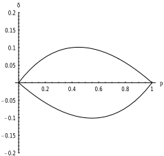
For a Bayesian network, the amount of permissible change is determined by Inequality 10, and is plotted in Figure 2. We can see that the amount of permissible change is small when the parameters have extreme values close to 0 or 1, because the relative odds change is large when even a very small absolute change is applied.
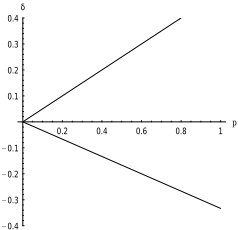
On the other hand, for a Markov network, the amount of permissible change is determined by Inequality 12, and is plotted in Figure 3. We can see that the amount of permissible change is proportional to the parameter values, because relative change is used instead of relative odds change.
Therefore, for a Bayesian network, the sensitivity of the network with respect to a parameter is largest for extreme values close to 0 or 1, and becomes smaller as the parameter approaches .5, while for a Markov network, the sensitivity of the network with respect to a parameter is proportional to its value, and increases as it grows larger.
The distance measure is useful in many aspects of sensitivity analysis. For example, given the possible single parameter changes in our example in the previous section, we can choose the one which perturbs the network the least according to the distance measure. In this case, the most preferred single parameter change is to decrease the parameter θa2, ¯ b1 from 2 to .533, incurring a distance measure of 1.322.
Moreover, we can also use the distance measure to find the optimal solution for changing all parameters in a clique table, which is the solution that satisfies Inequality 5 and minimizes the distance measure. As the distance measure D(ΘC,Θ′C) is computed using the maximum relative change in the parameters, the relative changes in all parameters must be the same for the optimal solution, because to obtain another solution that satisfies the constraint, we must increase the relative change in one parameter while decreasing the relative change in another, thereby incurring a larger distance measure.
For example, in our example from the previous section, to ensure our query constraint, we would like to decrease the parameters θa2,b1 and θa2, ¯ b1 and increase the parameters θ ¯ a2,b1 and θ ¯ a2, ¯ b1 , such that the relative changes in all parameters are the same. However, since only the ratios between the parameters are important, we can keep the first two parameters constant and only increase the last two parameters. The optimal solution of Inequality 5 is:
This parameter change incurs a distance measure of .350. It involves all parameters in the clique table and incurs a smaller distance measure than any of the single parameter changes computed earlier.
Finally, if we change the parameters in different clique tables which do not share any variables, the distance measure can be computed as the sum of the local distance measures between the clique tables. This result is also similar to the case of Bayesian networks [Chan and Darwiche, 2004].
5 Conclusion
In this paper, we expanded some of the main results in the topic of sensitivity analysis from Bayesian networks to Markov networks. We were able to find many parallels between the results in both models even given the differences in how their parameters are interpreted. Our results allow for the effective debugging of Markov networks by changing parameters in a single potential for ensuring query constraints. We also showed how to compute a bound on any query change between two Markov networks that have the same structure, but differ in the parameters of a single potential, and to choose parameter changes which minimize network disturbance. Finally, we identified a key semantical difference between Bayesian networks and Markov networks, relating to how parameter changes should be quantified.
@inproceedings{ijcai2005p95,
  title     = {Sensitivity Analysis in Markov Networks},
  author    = {Chan, Hei and Darwiche, Adnan},
  booktitle = {Proceedings of the Nineteenth International Joint Conference on
               Artificial Intelligence, {IJCAI-05}},
  publisher = {International Joint Conferences on Artificial Intelligence},
  editor    = {Leslie Pack Kaelbling and Alessandro Saffiotti},
  pages     = {1300--1304},
  year      = {2005},
  url       = {https://ijcai.org/proceedings/2005/95},
}
TY - CPAPER TI - Sensitivity Analysis in Markov Networks AU - Chan, Hei AU - Darwiche, Adnan T2 - Proceedings of the Nineteenth International Joint Conference on Artificial Intelligence, IJCAI-05 PB - International Joint Conferences on Artificial Intelligence PY - 2005 SP - 1300 EP - 1304 UR - https://ijcai.org/proceedings/2005/95 ER -Copied
Machine-readable versions of this paper, for tools and AI agents:





