
Efficient Distributed "Hormone" Graph Gradients
Proceedings of the Nineteenth International Joint Conference on Artificial Intelligence. Pages 1489-1493.
© 2005 International Joint Conferences on Artificial Intelligence
Abstract
Several researchers have attempted extract the principles behind hormone gradients found in biological system, and apply them to control physically manifested distributed systems. This paper presents an efficient implementation of a graph-based version of hormone gradient mechanisms. The algorithm is based on hop-counting of the topological distance between any given vertex and the hormone emitting vertex, and can deal with dynamic changes to the topology of the system. Performance of the described algorithm is documented through a number of experiments. The algorithm was developed for use in self-reconfigurable robotics, but might very well be useful for many other applications. The use of the algorithm to provide a common coordinate system for a collection of selfreconfigurable robot modules is described, that provides pose relative to the emitting module for all modules affected by the hormone.
- [Abelson et al., 2000] H. Abelson, D. Allen, D. Coore, C. Hanson, G. Homsy, T. Knight, R. Nagpal, E. Rauch, G. Sussman, and R. Weiss. Amorphous computing. Com- munications of the ACM, 43(5):74-82, 2000.
- [Bojinov et al., 2000] H. Bojinov, A. Casal, and T. Hogg. Multiagent control of self-reconfigurable robots. In Fourth International Conference on MultiAgent Systems (IC- MAS), pages 143-150, Boston, Massachusetts, USA, July 2000.
- [Butler et al., 2002] Z. Butler, K. Kotay, D. Rus, and K. Tomita. Generic decentralized control for a class of self-reconfigurable robots. In Proceedings, IEEE Int. Conf. on Robotics and Automation (ICRA), volume 1, pages 809-815, Washington, DC, USA, 2002.
- [Gafni and Bertsekas, 1981] E. Gafni and D. P. Bertsekas. Distributed algorithms for generating loopfree routes in networks with frequently changing topology. IEEE Trans. on Comm., COM-29:11-18, 1981.
- [Hotz, 2004] P. E. Hotz. Asymmetric cell division in artifi- cial evolution. In Congress on Evolutionary Computation (CEC), 2004.
- [Meinhardt and Gierer, 2000] H. Meinhardt and A. Gierer. Pattern formation by local self-activation and lateral inhi- bition. Bioessays, 22(8):753-60, Aug 2000.
- [Meinhardt, 1993] H. Meinhardt. A model for pattern for- mation of hypostome, tentacles, and foot in hydra: how to form structures close to each other, how to form them at a distance. Developmental Biology, 157(2):321-333, June 1993.
- [Nagpal et al., 2003] R. Nagpal, A. Kondacs, and C. Chang. Programming methodology for biologically-inspired self- assembling systems. In Proceedings, AAAI Spring Sym- posium on Computational Synthesis: From Basic Building Blocks to High Level Functionality, 2003.
- [Nagpal, 1999] R. Nagpal. Organizing a global coordinate system from local information on an amorphous computer. AI Memo 1666, 1999.
- [Nishimura and Sasai, 2004] S. I. Nishimura and M. Sasai. Chemotaxis of an eukaryotic cell in complex gradients of chemoattractants. In The ninth international symposium on artificial life and robotics (AROB), Beppu, Oita, Japan, January 2004.
References were extracted automatically from the PDF and may contain errors.
Full text extracted automatically from the PDF; figures, tables and equations may differ. The PDF is the version of record.
1 Introduction
Hormone gradients have a central role in the coordination of growth and self-repair in biological multicellular systems. Several researchers have attempted to use these same mechanisms to control physically manifested distributed systems, by using some abstraction over the perceived functioning of biological hormone gradients. This paper presents an ef�cient implementation of a graph-based version of hormone gradient mechanisms, based on hop-counting and spanning a tree over the topology, that can deal with dynamic changes to the topology of the system. The paper will also describe how the algorithm can be used to relay a common coordinate system for modules in a self-recon�gurable robot. Even though the focus was on self-recon�gurable robots during development, the algorithm is believed to have much wider applicability.
2 Graph-Based Hormone Gradients
As a �rst approximation, simple gradients are fairly easy to implement. Figure 1 illustration a) shows a graph representing a system of 11 vertices, with 11 edges. In b) a simple width �rst graph traversal algorithm (starting at the gray vertex) has been applied to assign a value to each vertex, where the value corresponds to the recursion depth. The result is that each vertex holds its distance to the gray vertex. In c) a similar algorithm is run, where a limit has been imposed on the recursion depth. The value assigned to vertices is the limit minus the recursion depth, resulting in the held value decreasing the further we get away from the gray module. This can be regarded as an abstract implementation of a hormone gradient emitted from the gray vertex. The hormone gradient is emitted with a given strength that de�nes the depth of the recursion (the maximum topological distance) and thus the number of affected vertices. The c) approach also allows us to have several emitting vertices, as shown in d) where two vertices are emitting a gradient, one with strength 3, and one with strength 5. In d) the graph algorithm is designed such that once a vertex has been assigned a value, only higher values can be assigned to that vertex.
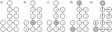
To illustrate how this can be used as a gradient, in e) arrows point to the edge leading to the vertex with highest value. We see that if we start at any vertex in the graph and follow the arrows, we end up at one of the emitting vertices. Also we see that the vertex with a higher emission strength has a larger basin of attraction than the vertex with lower emission strength.
3 Agent-Based Hormone Gradients
The previous section brie�y described how traditional graph traversal algorithms can produce a loose analogy to biological hormone gradients. However, in a physically distributed system we cannot directly use graph traversal algorithms.
This paper presents a distributed algorithm, providing information on topological distance in communication networks with dynamic changing topologies. Consider an agent for each vertex in the graph, where agents asynchronously and without any global knowledge, ef�ciently realizes such graph hormone gradient information.
3.1 RelatedWork
Hormone gradients have been studied by biologists and have been found to be a key player in coordinating and controlling growth in plants and animals. Mainhardt and Gierers' [Meinhardt, 1993] [Meinhardt and Gierer, 2000] work on how hormone gradients control the forming of the tentacles of the Hydra animal describes how hormones are responsible for almost all aspects of shaping the animals body. Other relevant work includes Nishimura's [Nishimura and Sasai, 2004] work on chemo-taxis on cells in solutions with chemical gradients.
All the implementations of digital hormone gradients in the distributed robotics literature rely on continuous broadcasting of a hop-count number. When an agent receives a message with a hop count number, it remembers this number and starts emitting a message with an incremented or decremented hop count number, at regular intervals. A timer keeps track on when the last message matching the stored hop count number was received. If too long time has expired, the stored hop count number is erased, and the agents stop sending messages.
Several researchers have extracted and abstracted these mechanisms for use in the multi-robot domain. Amorphous computing [Abelson et al., 2000][Nagpal, 1999][Nagpal et al., 2003] is one example of research relying heavily on simulated hormone gradients, and many more examples exist, including work on cell division in arti�cial evolution [Hotz, 2004], and in self-recon�gurable robotics, such as Bojinov, Casal and Hogg's scents [Bojinov et al., 2000].
As a �rst approximation, this continuous broadcasting approach works �ne. However, there are two main problems with this approach:
- Frequent emission of messages, even if there is no change to the topology of the agents.
- Continuous broadcast style approaches can fail to deal adequately with dramatic changes to the topology.
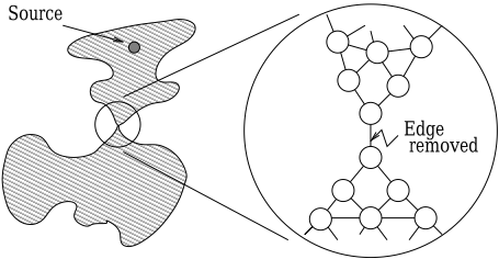
The �rst point has to do with ef�ciency in terms of power consumption and processing power. The second point, illustrated in �gure 2, is more serious.
For these two reasons, it is desirable to develop a better algorithm.
4 Features of the Algorithm
The algorithm described in this paper is an extension of E. Gafni and D. Bertsekas' work described in the paper �Distributed Algorithms for Generating Loopfree Routes in Networks with Frequently Changing Topology� [Gafni and Bertsekas, 1981]. Their algorithm has a number of properties that makes it interesting for the purpose of this paper:
- The algorithm is distributed and works on unknown communication topologies.
- Their algorithm spans a directed acyclic graph (DAG) over the network topology, where all directed paths lead to the destination.
- In the event of changes to the topology of the network, the algorithm creates a new DAG using an iterative method.
From a functional point of view, the algorithm presented in this paper is an improved version of the algorithm presented by Gafni and Bersekas, with two additional features;
- From a given vertex, the length of any directed path to the destination is equal to the shortest undirected path to the destination.
- Each vertex knows its topological distance from the destination.
4.1 Definitions
The algorithm described below works on a graph, to create a loose analogy to chemical/hormone gradients. The algorithm is completely distributed, and is able to deal with frequently changing topology, while at the same time using very little communication. Consider an agent for each vertex v in the graph G = (V,E). Agents have a number of ports, through which they can communicate to other agents. The algorithm uses two features per agent. Agents can emit a hormone with strength s and sense the intensity i of the hormone. Both s and i are in ✄ , the set of natural numbers. We require agents to know which of their ports are connected to other agents, and which are not. Given this, a digital hormone gradient can be de�ned as a four-tuple, {G, I, S, P}, where:
- G = (V,E) is a graph, where vertices are elements of the con�guration, and edges are physical connections between the elements.
- I : V → ✄ is the hormone intensity (concentration) mapping, so that i = I(v) is the hormone intensity for vertex v.
- S : V → ✄ is the hormone emission strength mapping, where s = S(v) is the strength s with which vertex v ∈ V emits the hormone.
- P : (V × ✄ ) → ({⋄} ⋃ V ) is the port function. The port function holds information for the state of each of the agent's ports, so that P(v, n) is the state of the agent for vertex v's n'th port. The symbol ⋄ is used to specify a port that is not connected, such that ∀n ∈ ✄ : ∀v ∈ V : ∀v′ ∈ P(v, n), {v, v′ } ∈ E ⇔P(v, n) ∈ V .
The four-tuple {G, I, S, P} describes the global state of the hormone gradient, but we are aiming at a distributed algorithm with only local information. For any given vertex v ∈ V , the local gradient state information available is i = I(v), s = S(v) and for each of the j ports, pn = P (v, n) where 0 ≤ n < j. Besides this information, the algorithm requires agents to remember their parent in the spanning tree -1 ≤ f < j (using -1 for no parent), a timer/counter t ∈ ✄ and an array for storing information on which ports to send messages to, m[n] ∈ {NONE, PROPAGATE}.
The algorithm basically works by maintaining local information on the spanning tree, such that the variable f always points to the port from which the gradient is �owing. The timer/counter is used to adjust the relative speeds of propagating gradient and deleting the gradient. Without this adjustment continuous propagation and deletion of the gradient in local cyclic areas of the graph might arise, causing much communication and slow hormone deletion. However, this adjustment introduces a parameter that is the number of time steps to delay propagate messages when spreading the gradient. Lower values cause the algorithm to be faster but more unstable.
The algorithm for each agent, implementing the desired graph-based hormone gradient behavior, is given below. Note that neither global communication nor synchronization between agents is assumed.
The -initialize- function resets the variables of the agent. -emitGradeint- is used to set the hormone emission strength of the agent. Setting to zero clears the gradient. -updateGradient- holds the central functionality such as sending messages, and should be called at regular time intervals. The frequency at which it is called determines the hormone propagation speed in the system. The four event functions -connectEvent-, -disconnectEvent-, -propagateMessageRecievedEvent- and -deleteMessageRecievedEvent- are very light-weight and can be called in some interrupt routine whenever the corresponding event is detected.
-initialize()- i := 0; s := 0; f := 0; t := 0; foreach n ∈ {0..j - 1} do m[n] :=NONE; end -emitGradient(s ′ )- s := s′ ; -connectEvent(n)- m[n] := PROPAGATE;-disconnectEvent(n)- if n = f then f := -1; end -updateGradient()- if s > i then i := s; f := -1; foreach n ∈ {0..j - 1} do m[n] := PROPAGATE; end else if s < i ∧ f = -1 then foreach n ∈ {0..j - 1} do if pn ̸= ⋄ then sendDeleteMessage(n,i-1); end m[n] :=NONE; end i := 0; else if t > 0 then t := t -1; if t = 0 then foreach n ∈ {0..j - 1} do if n ̸= f then m[n] := PROPAGATE; end end end else foreach n ∈ {0..j - 1} do if pn ̸= ⋄ ∧ m[n] = PROPAGATE ∧ i > 1 then sendPropagateMessage(n,i-1); t := 0; end m[n] :=NONE; end end -propagateMessageRecievedEvent(n ′ , i′ )- if i′ > i then i := i′ ; f := n′ ; t := 3;// This constant (3) de�nes the delay before propagating the gradient, to allow delete messages to �catch up�. else if i′ < i - 1 then m[n′ ] := PROPAGATE; end -deleteMessageRecievedEvent(n ′ , i′ )- if i′ ≥ i then f := -1; else m[n′ ] := PROPAGATE; end4.2 Tests of the Algorithm
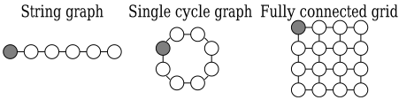
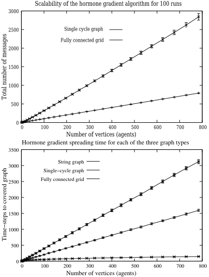
The algorithm was implemented and tested on graphs with varying sizes and numbers of loops, shown in �gure 3. To test the robustness of the algorithm, the different activation schemes described in [Butler et al., 2002], D0,D1 and D∞, were used for the agents. In D0, agents are activated in a �xed order each time step, in D1 the agents activation order is permuted for each time step, and in D∞ a random agent is picked and activated n times each time step, where n is the number of agents. Figure 4 shows the number of messages passed as a function of the number of modules for three different graph types, using the D∞ activation scheme. The data shows that the algorithm has good performance, in that the number of messages passed is linearly proportional to the number of edges in the graphs, and that the number of time steps used to propagate the hormone is proportional to the diameter of the graph.
A different set of experiments were performed for counting the number of messages used to remove the gradient again, by setting the emission strength of the emitting agent to zero. These results are shown in �gure 5. The results show that the number of messages generated for removing a hormone is linearly proportional to the number of involved graph edges. Notice that removing the hormone is faster than covering the graph, due to the delay on propagating the gradient.
5 Pose Hormone Gradients
The previous section described the basic graph hormone gradient algorithm. This section describes how the algorithm has been used for controlling two self-recon�gurable robot systems, shown in �gure 6. Self-recon�gurable robot control is a good application test bed for this kind of hormone gradient algorithms, because of the constantly changing topology in such a robot, and because of similarities between selfrecon�gurable robots and multi-cellular organisms.
5.1 Common Pose for Self-Reconfigurable Robot Modules
The distributed hormone gradient algorithm described above can be expanded slightly to be used for propagating pose (position and orientation) relative to the emitting vertex in a self-recon�gurable robot. Basically, the expanded algorithm uses feed-forward kinematics in the generated directed acyclic graph to compute the relative pose to the emitting vertex. To realize this, it is a requirement that the relative pose between two connected vertices in the con�guration can be found. We let the space a0 be the space of relative poses in a 3D vector space.
Then, a relative pose hormone is a four-tuple, {G, I, S, P} where:
- G = (V,E) is a graph, where vertices are elements of the con�guration, and edges are physical connections between the elements.
- I : V → (✄ × a0 ) is the hormone intensity (concentration) mapping, so that i = I(v), i = 〈in, ip〉, where in ∈ ✄ , ip ∈ a0 is the hormone intensity in and relative pose ip for vertex v.
- S : V → (✄ × a0 ) is the hormone emission mapping, where s = S(v), s = 〈si, sp〉 is the emission strength (si) and the emitted pose (sp) for vertex v.
- P : (V × ✄ ) → ({⋄} ⋃(V × a0 )) is the port function. The port function holds information for the state of each of agent's ports, so that P(v, n) is the state of vertex v's n'th port. The symbol ⋄ is used to specify a port that is not connected, such that ∀n ∈ ✄ : ∀v ∈ V : ∀〈v ′ , p′ 〉 ∈ P(v, n) : {v, v′} ∈ E ⇔ P(v, n) ∈ V . Here, p′ is the relative orientation between the two connected elements, such that if pv′ is the pose of v′ and pv is the pose of v, then pv′ × p′ = pv.
For any given module v ∈ V , the local gradient state information available is i = 〈in, ip〉 = I(v), s = 〈si, sp〉 = S(v) and for each of the modules j connectors, pn = P(v, n) is either ⋄ or 〈v′ , p′ 〉, for 0 ≤ n < j.
The principle is to do feed-forward kinematics in the directed acyclic graph generated by the graph hormone algorithm. As a consequence, each module affected by the hormone knows its relative position and orientation to the hormone source. It turns out that by exploiting that each module knows its relative position to the source, it is possible to re- Number of vertices move the delay for propagate messages by adding an extra condition for the case of receiving a propagate message. The implementation details of the pose hormone gradient algorithm has been omitted due to space constraints.
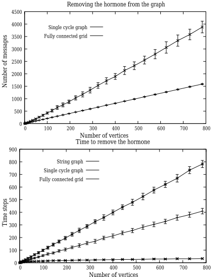
Figure 5: Tests on removing the hormone from the graph by setting the emission strength of the emitting vertex to zero, after the hormone has fully propagated. The two graphs show the number of messages generated and the time used for the three graph families and for varying graph sizes. In the top graph the string graph results were omitted since they are identical to the single cycle results. Notice that removing the hormone is faster than propagating the hormone, but produces more communication and has higher variance. This relationship can be adjusted by changing the propagation delay.
6 Implementation and Experiments
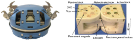
The pose hormone algorithm has been implemented and tested on simulations of the ATRON system, �gure 6, left, and on the M-TRAN system, �gure 6, right.
Both the ATRON and the M-TRAN modules are composed of two parts, where the parts are connected by an actuated joint. The algorithm is implemented, such that each part of the modules corresponds to a vertex in the graph. The following will describe some experiments done on the pose hormone algorithm on the simulated M-TRAN robots.
6.1 M-TRAN, Message Count
Three test con�guration designs are shown in �gure 7. Each con�guration comes in a form with 4, 32, 108, 256, 500 and
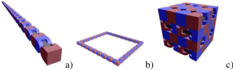
864 modules. The three designs differ in the number of loops in the topology, where a) has no loops, b) a single loop and c) has many loops.
An experiment proceeds as follows:
- A module in one end/corner is set to emit a hormone gradient with an emission strength of 1000.
- Data is collected on the number of messages used to fully propagate the gradient, and on how many time steps it took.
- Then the emission strength of the emitting module is set to zero.
- Similarly to step two, data is collected.
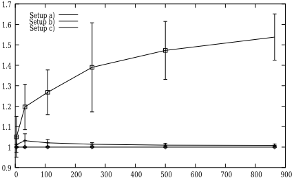
The algorithm was tested using the D0, D1 and D∞ activation schemes. Ten experiments were performed for each combination of con�guration and activation scheme, and mean and variance were computed. The correctness of the pose information is easily veri�ed by placing the emitting module such that the emitted pose is identical to the pose in the simulator. In this case, the relative pose hormone for any module should be identical with its pose in the simulator (provided appropriate scaling). Figure 8 shows the average number of messages, and �gure 9 the communication load per connector, using the D1 activation scheme. For deleting the hormone gradient, the number of messages passed by any connected connector was constant two.
Besides these simple tests, the algorithm was used a lot during work on control of the two self-recon�gurable robot systems, to produce a common coordinate frame of reference for locally cooperating groups of modules.
7 Discussion &Conclusion
This paper describes an ef�cient algorithm for realizing an abstract implementation of hormone gradients. Hormone gradients are widely used in biology to coordinate and differentiate cellular behavior.
| Test Con�guration | a) | b) | c) | ||||||
|---|---|---|---|---|---|---|---|---|---|
| # modules | 4 | 32 | 108 | 4 | 32 | 108 | 4 | 32 | 108 |
| # connections | 3 | 31 | 107 | 4 | 32 | 108 | 4 | 64 | 252 |
| # messages for propagating | 7 | 63 | 210 | 8 | 66 | 221 | 9 | 115 | 455 |
| # message for deleting | 14 | 126 | 420 | 16 | 128 | 432 | 16 | 193 | 720 |
The described algorithm is based on topological distance, and is capable of dealing with changing topology in the connectivity graph using only local information and without requiring global synchronization.
The algorithm has properties similar to that of Gafni and Bertsekas, with the added bene�t that the spanning DAG is, in a sense, optimal, in that any directed path tho the source has the same length as the shortest undirected path. Additionally, in contrast to the commonly used continuous broadcast method, the presented algorithm only generates communication when the topology of the graph changes, or when the gradient information changes. Furthermore, only a constant (and small) number of messages is generate per graph edge, in the event of any change to the hormone gradient. Less communication results in reduced hardware requirements, that again can reduce requirements to power, processing, price and size.
Performance of the described algorithm is documented through a number of experiments. An expansion of the hormone gradient algorithm is given which can be used to provide all self-recon�gurable robot modules affected by the hormone their pose relative to the emitting module. The algorithm was developed for use in self-recon�gurable robotics, but might very well be useful for many other applications. Future work will include further analysis of performance and analytical proofs.
@inproceedings{ijcai2005p23,
  title     = {Efficient Distributed "Hormone" Graph Gradients},
  author    = {Østergaard, Esben Hallundbæk},
  booktitle = {Proceedings of the Nineteenth International Joint Conference on
               Artificial Intelligence, {IJCAI-05}},
  publisher = {International Joint Conferences on Artificial Intelligence},
  editor    = {Leslie Pack Kaelbling and Alessandro Saffiotti},
  pages     = {1489--1493},
  year      = {2005},
  url       = {https://ijcai.org/proceedings/2005/23},
}
TY - CPAPER TI - Efficient Distributed "Hormone" Graph Gradients AU - Østergaard, Esben Hallundbæk T2 - Proceedings of the Nineteenth International Joint Conference on Artificial Intelligence, IJCAI-05 PB - International Joint Conferences on Artificial Intelligence PY - 2005 SP - 1489 EP - 1493 UR - https://ijcai.org/proceedings/2005/23 ER -Copied
Machine-readable versions of this paper, for tools and AI agents:





