Temporal-Difference Networks with History

Tanner, Brian; Sutton, Richard S.

Temporal-Difference Networks with History

Download BibTeX Cite

Proceedings of the Nineteenth International Joint Conference on Artificial Intelligence. Pages 865-869.

Abstract

emporal-difference (TD) networks are a formalism for expressing and learning grounded world knowledge in a predictive form [Sutton and Tanner, 2005]. However, not all partially observable Markov decision processes can be efficiently learned with TD networks. In this paper, we extend TD networks by allowing the network-update process (answer network) to depend on the recent history of previous actions and observations rather than only on the most recent action and observation. We show that this extension enables the solution of a larger class of problems than can be solved by the original TD networks or by historybased methods alone. In addition, we apply TD networks to a problem that, while still simple, is significantly larger than has previously been considered. We show that history-extended TD networks can learn much of the common-sense knowledge of an egocentric gridworld domain with a single bit of perception.

[Jaeger, 1998] Herbert Jaeger. Discrete-time, discrete-valued observable operator models: a tutorial. Technical report, German National Research Center for Information Tech- nology, 1998.
[Littman et al., 2002] M.L. Littman, R. S. Sutton, and S. Singh. Predictive representations of state. In Advances in Neural Information Processing Systems 14, Cambridge, MA, 2002. MIT Press.
[Rosencrantz et al., 2004] Matthew Rosencrantz, Geoff Gor- don, and Sebastian Thrun. Learning low dimensional pre- dictive representations. In ICML '04: Twenty-first interna- tional conference on Machine learning. ACM Press, 2004.
[Singh et al., 2004] Satinder Singh, Michael R. James, and Matthew R. Rudary. Predictive state representations: A new theory for modeling dynamical systems. In Uncer- tainty in Artificial Intelligence: Proceedings of the Twen- tieth Conference, pages 512-519, 2004.
[Singh, 2004] Satinder Singh. Private communication, 2004.
[Sutton and Tanner, 2005] Richard S. Sutton and Brian Tan- ner. Temporal-difference networks. In Advances in Neu- ral Information Processing Systems 17, pages 1377-1384, Cambridge, MA, 2005. MIT Press.

References were extracted automatically from the PDF and may contain errors.

Full text extracted automatically from the PDF; figures, tables and equations may differ. The PDF is the version of record.

1 TDNetworks without History

In the following text we describe a specific instantiation of the original TD networks specification that is instructive for understanding the details of our work. For information on the general specification of TD networks we direct the reader to the original work [Sutton and Tanner, 2005].

The problem addressed by TD networks is a general one of learning to predict aspects of the interaction between a decision making agent and its environment (a dynamical system). At each of a series of discrete time steps t, and agent takes an action at ∈ A and the environment responds by generating an observation ot ∈ O. In this work, we will consider TD networks with two observations, 0 and 1. The action and observation events occur in sequence, at-1, ot, at, ot+1, at+1, ot+2. This sequence will be called experience. We are interested in predicting not just each next observation, but more general, action-conditional functions of future experience.

The focus of this work current is on partially observable environments-environments where the observation ot is not a sufficient statistic to make optimal predictions about future experience (ot does not uniquely identify the state of the environment). We will be using TD networks to learn a model of the environment that is accurate and can be maintained over time.

A TD network is a network of nodes, each representing a single scalar prediction. The nodes are interconnected by links representing target relationships between predictions, observations, and actions. These nodes and links determine a set of questions being asked about the data and predictions, and accordingly are called the question network.

Each node on the TD network is a function approximator that outputs a prediction using inputs such as the current observation, the previous action, and the predictions made at the previous time step. This computation part of the TD network is thought of as providing the answers to the questions, and accordingly is called the answer network.

Figure 1 shows a typical question network. The question of node y0 at time t is 'If the next action is a1, what is the probability that the next observation ot+1 will be 1?'. Similarly, node y2 asks 'If the next action is a1, what will node y0 predict at time t + 1?'. This is a desired relationship between predictions, but also a question about the data. We can unroll this interpredictive (or TD) relationship to look at the extensive relationship between y2 and the data, which yields the question 'If the next two actions are a1, what is the probability that ot+2 will be 1?'.

In a fully observable (Markov) environment, it is natural for the question network to be a set of questions that are in some way interesting to the experimenter. In partiallyobservable environments the structure of the question network has additional constraints; the answers should be a sufficient statistic that accurately represents the state and can be updated as new data becomes available. Although the question of how to discover a question network that expresses a minimal sufficient statistic is important, it is tangental to the focus of this work. The question networks we use are not minimal, and a network like that in Figure 1 likely contains extraneous questions.

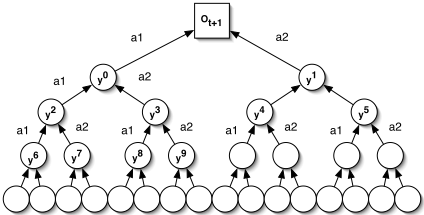
Figure 1: Symmetric action-conditional question network. The network forms a symmetric tree, with a branching factor of |A|. This example has depth d = 4. Some of the labels have been left out of this diagram for clarity, each of these nodes should have a label yi and each is conditioned on some action.

Formally, yi t ∈ [0, 1], i = 0, . . . , n - 1 denotes the prediction for node i at time step t. The column vector of predictions yt = (y0 t , . . . , yn-1 t )T is updated according to a vectorvalued prediction function with modifiable parameter W:

Formula not decoded

This prediction function corresponds to the answer network, where xt ∈ ℜm is a feature vector, Wt is a n × m matrix of weights, and σ is the S-shaped logistic function σ(s) = 1 1+e-s . The feature vector is a function of the preceding action, observation, and node values.

In previous work on TD networks, xt had a binary component for each unique combination of the current observation and previous action (one of which is 1, the rest 0), and n more for the previous node values yt-1 . Additionally, xt has a bias term (constant value of 1). In our experiments we also included real valued features with the complement of the predictions from the last time step (1 - yt-1 ), although we later found this was not necessary. The learning algorithm for each component wij t ofWt is of the form

Formula not decoded

where α is a step-size parameter, zi t is a target for yi defined by a question network, and cit ∈ {0, 1} corresponds to whether the action condition for yi was met at time t.

2 Cycle-World Counterexamples

In our experimentation we found that TD networks are able to solve certain, but not all of our small testing problems. The success of learning does not seem to be directly correlated with the complexity of the environment. In previous work, TD networks were able to learn an accurate model of a partially-observable seven-state deterministic random walk as well as the probabilities in a fully observable stochastic random walk [Sutton and Tanner, 2005]. Since that time, we have discovered that TD networks are unable to learn an accurate model of certain small partially-observable deterministic environments. Careful analysis has determined that the question networks that were used were sufficient to represent the appropriate model, so the issue must lie somewhere in the TD network specification.

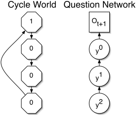
Figure 2 presents a simple example of a task and question network for which the solution is representable but not learnable by TD networks without history. The cycle world consists of the four states shown on the left. The current state of the system cycles clockwise through the states. There is a single observation bit that is 1 at the top of the cycle, and 0 at all other times. On the right is a question network which asks what the observation bit will be one, two, and three time steps in the future. Recall that at time t, yt is calculated as a function of (yt-1 , at-1, ot,Wt). If we assume that the yt-1 is correct, there is a solution for the weights that will keep yt correct at each successive time step. Unfortunately, yt-1 will never be correct; the solution exists but will not be found.

To illustrate this, we must look at the question network, and remember that it specifies target values for the answer network. At the start of training, yt-1 will be likely be incorrect. There are no actions in this environment, so the current observation ot is the only useful input feature in xt. For the network to become correct, it is necessary that some sequence of questions can eventually be answered, starting or anchored only with knowledge of ot. Also note that when training begins, the only node with a valid target is y0 , because its target is not a prediction, but rather the grounded observable value of ot+1. As training progresses, the agent interacts with the environment and some answers will be learned, anchored only on the grounded observations. Eventually, the environment will reach a point where ot = 0 and y0 t should be 1. The information that distinguishes this case from the case where ot = 0 and y0 t should be 0 lies in a correct answer for y1 t-1 . Unfortunately, the target for y1 t-1 is y0 t . In this case, the cyclic dependency between the question network and the temporal flow of information eliminates the possibility of the TD network learning a correct solution.

After considering this problem, it became apparent that it is necessary to find an augmentation to the TD network specification to eliminate cyclic information dependencies. Such a dependency occurs when the target zi for node i relies on yi making accurate predictions. This dependency can be eliminated by providing additional input features to the TD network. This additional information acts as an anchor for the TD network predictions.

Incidentally, good approximate solutions to the cycle world can be learned by TD networks consisting of a single node. Clearly, there is no way that a single predictive node can solve this problem perfectly, but it can achieve very low error in an unusual way. When ot = 1, the network predicts approximately .001. On the next time step, the network will multiply the previous prediction so as to predict approximately .01. On the next step it will predict .1, and then finally .99 for the step where ot will again be 1. Unfortunately this solution is not stable, and continued training leads to oscillation between this sort of approximate solution and strictly predicting 0 at each step.

Figure 2: A counterexample for TD-network learning without history. On the left is a representation of the cycle world. This environment has four states that are cycled through deterministically. On the right is the associated question network. There are no actions in this world.

Figure 3: Input vector for cycle world with 3-step history and 3 levels of predictive nodes. On the left is the definition of each feature. The first feature is the bias term. The next 8 features correspond to the 8 distinct 3-step histories {ot-2ot-1ot} (not all are possible in this world). The final 3 features are the predictions from the previous time step. The middle vector is a sample input vector for the third state from the top of the cycle world at the start of learning. At this point, all of the predictions are at their initial value, .5. Finally, the rightmost vector is the input vector for the third state when learning is complete, all of the predictions are accurate.
Features	Initial	Final
1 history = 000 history = 001 history = 010 history = 011 history = 100 history = 101 history = 110 history = 111 y 0 t-1 y 1 t-1 y 2 t-1	1 0 0 0 0 1 0 0 0 .5 .5 .5	1 0 0 0 0 1 0 0 0 0 0 1

3 TDNetworks with History

The cycle world is a problem in which there is a simple relationship between the observations and recent experience. Methods that try to directly learn such relationships are called history-based methods. We will consider history-based methods which predict ot+1 using a different variable for each unique k-length window of history where a k-length window of history is defined as at-kot-k+1...at-1ot. In this case, a window of length 3 would be sufficient to uniquely identify each state of the system and thus would be able to make accurate predictions. Incorporating short history into the feature vector xt of a TD network should allow the TD network to learn a correct solution to this problem. Figure 3 shows an example of a hybrid input vector that uses 3 time steps of history and 3 predictive nodes.

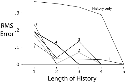
In order to test the hypothesis that incorporating history into the input vector xt of a TD network would allow it to solve a greater class of problem, we used a cycle world like that in Figure 2, except with six states instead of four. This size was chosen to clearly illustrate the effectiveness of different configurations of history and predictive nodes. On this problem, we tested three different methods: (1) TD networks as previously specified without history, (2) a simple historybased approach, (3) a combination of TD networks and history together. For each method we used several values for the step size parameter; the best of these was used as the performance measure for that method. For each method and step size, the network was trained for at least one million time steps. The 1-step prediction errors were averaged over the final 20000 steps to produce an overall performance measure for each method.

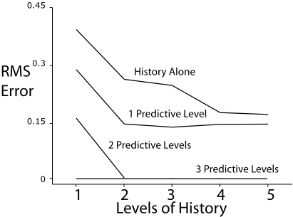
The results, shown in Figure 4, show that the simple history-based method only performed well when it had enough history to solve the problem exactly. TD networks without history correspond to the data points with history length one. These performances are better than history of length one, but not as good as the TD networks with history. It is also interesting to notice that the TD network is able to solve the problem with a much shorter window than the history-based method alone. This illustrates that our combined algorithm is not simply using history instead of the predictive representation, but rather is leveraging the history to learn a predictive representation. It is interesting that the performance of the various combinations of history and predictive nodes do not follow a clear pattern. For example, when there are 2 predictive nodes, it appears that 2 or 4 steps of history is better than having 3 steps. We have verified that the minimum length of history required to solve the 6-state cycle world exactly with 2 predictive nodes is a 4-step history. This means that the low error seen with 2 steps of history is a case of the TD network stumbling on a good approximate solution when it could not represent an exact solution (as discussed at the end of Section 2).

Figure 4: Performance on the 6-state cycle world of TD networks extend to incorporate various lengths of history. The different lines correspond to different depths of the question network, as indicated by the numeric label.

4 Indefinite-memory Problems

In the previous section, we introduced history to the TD network specification in order to eliminate cyclic dependencies and increase the class of problems where solutions can be learned with TD networks. There appeared to be a tradeoff between predictive levels in the question network and lengths of history. From this example alone, it may not be clear that the combined approach is superior to a history-only approach. There is a potentially large class of problems that cannot be represented with a history-only approach, but can be represented and solved by TD networks. Environments in this class are such that there is no finite length of history that State C

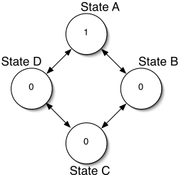
Figure 5: An indefinite-memory problem, the four-state deterministic ring world. There are two actions in this world, next and previous. Next advances in clockwise rotation while previous advances in counter-clockwise rotation. Prediction methods using a finite length history will lose localization after some number of transitions back and forth between states B and C or C and D.

can uniquely identify the current state of the environment. We will refer to problems in this class as indefinite-memory problems.

One simple example of an indefinite-memory problem is the ring world shown in Figure 5. Because states B, C, and D are indistinguishable, there are sequences of actions that keep the environment in that subset of states and will eventually fill a fixed-length memory with useless information. In contrast, a TD network can easily represent this environment, and can never be made to forget its location in the environment.

We applied TD networks with various depths of question network and lengths of history to the 5-state ring world problem. The performance measure used was the same as in the previous experiments, except in this case averaged over 25 independent runs of 10 million time steps. The results are shown in Figure 6. As the history window increases, the history-only method more closely approximates the correct solution. This improvement seems to diminish as the history window gets larger, and is further hampered by the fact that the number of unique histories grows exponentially with the length of the window. With the predictive approach, the problem is solved correctly with only 1 level of history and a predictive question network of depth 3.

It is interesting that, provided enough time, the TD network can learn a correct model of this environment without history, something which it could not do for the cycle world. Especially puzzling was that these two problems seemed highly related, the cycle world seemingly even less complex than the ring world. The fact that actions have inverses in the ring world eliminates the information flow dependencies that existed in the cycle world. In the ring world, the agent can incrementally learn more and more about the environment. In early training, the agent can anchor itself when ot = 1 because this observation uniquely identifies this state. As time passes, the agent can learn accurate 1-step predictions from that anchored location. It can also learn 2-step predictions that involve leaving this position and then returning immediately. This process can continue until this chaining effect has allowed the agent to make accurate predictions from all positions in the network.

Figure 6: Performance on the 5-state ring world as a function of length of history and depth of question network. The history method suffers from diminishing returns as size of the history window increases. Learning also slows considerably because the number of unique histories that can be observed grows exponentially.

5 Gridworld Experiments

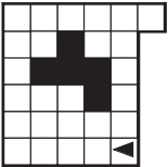
In previous work, and so far in this paper, TD networks have been applied only to abstract problems with fewer than 10 states. In this final section of the paper we present suggestive results for a gridworld environment that is an order of magnitude more complex than those previously considered. The gridworld in Figure 7 shows the environment that we chose. In this environment, the agent has a single perceptual input, a single bit indicating whether there is a wall directly in front of it. The agent also has a very limited action space, it can either attempt to move forward or it can rotate 90 degrees clock-wise. We encourage the reader to consider two analogous tasks suitable for a human. First, consider sitting at a table with two buttons and a light bulb. You are told that the light bulb will turn on and off based on the buttons pressed according to some unobservable process. If that unobservable process were the map in Figure 7, could a human learn this problem?

A second interpretation of the problem which should be more familiar is navigating around a room with the lights off. At all times you can feel if you are touching a wall, otherwise nothing. What sorts of common-sense knowledge would you apply to this type of scenario? The simplest knowledge is that if you are touching a wall and you attempt to walk forward, you will still be touching a wall. You would also know that 4 consecutive 90 degree turns ends with the same observation that it started with. These are the types of knowledge that can be learned easily with a history-based approach.

Figure 7: The gridworld used in the final experiment. The agent's location is represented by the triangle. The agent has a very limited perceptual space, it observes 1 if the arrow is pointing at a block, and 0 if the arrow is pointing at an open space. This agent has only two actions, forward and turn. Forward will move the agent 1 space in the direction that the arrow points (if it is not blocked), while turn will rotate the arrow clock-wise 90 degrees. There are 104 unique environmental states in this world.

There are other types of common-sense knowledge that are harder to learn with history. If you are facing wall, then you turn around (180 degrees), observe no wall and walk forward; what common-sense predictions could we make? First, we would know that turning 180 degrees again will be clear, and walking forward from there will take us back to the wall. We also know that if we rotate 360 degrees any number of times at any step of this process, the entire process remains intact, nothing changes. This concept is impossible to learn with a fixed length history. This scenario exemplifies the conceptual and practical difference between predictive representations and history-based representations. After facing a wall, turning 180 degrees and going forward, a 3-level history-based approach knows 'I am in the state described as {wall, turn, clear, turn, clear, forward, clear}'. The predictive agent has a different representation, more like 'I am in the state where{Pr(clear|turn, turn) = 1, P r(wall|turn, turn, forward) = 1, etc.}'.

We ran a TD network of depth 5 with a history of length 6 in this environment for more than 50 million time steps to give it the opportunity to learn about the causal structure of its environment. At the end of this time we took control of its decisions to explore particular places in the world as shown in Figure 8. On the left, this figure shows the state of the environment at various points in time as the agent is controlled from state to state. On the right a representation of the agents predictions at each step is shown. These predictions show that the agent has learned a great deal about its environment.

At t = 0 the agent is in a corner, and we can see that it knows there is a wall on its left side and a wall behind it. Notice just to the right of the 'A' is a dark bar. This bar represents the prediction for turning right, going forward twice, and then turning right three more times. The fact that this bar is dark indicates that the agent correctly knows something about the nearest interior blocked cell. Above the 'A', the agent also predicts a wall and below the 'A' it predicts gray. This shows that the agent does not completely understand that it will be blocked if it chooses forward, turn forward, but it surely knows it will be blocked if it went forward again at the end of that sequence.

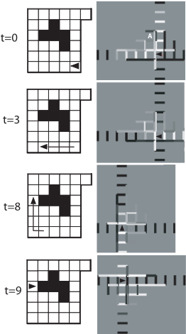
Figure 8: A sample trajectory in the gridworld and a representation of the associated predictions at several time steps. The representation of the agent's predictions is laid out as a subjective action-conditional map of the area near the agent. All of the colored bars correspond to some prediction that the agent is making. For example, if the agent believes that it will observe a wall by going forward, the bar in front of the triangle of it is black. If the agent believes it will be clear, the bar is white, and if the agent is uncertain, the bar is gray.

The white bars in front of the agent indicate that it believes it will see clear if it goes forward for the next four steps, and then it will see a wall.

At t = 3, the agent has moved along the wall and we can see that its expectation of seeing a wall ahead of it has moved closer, while to its left are all the predictions appropriate to their being an extended wall.

At t = 8, the agent has moved along another wall. Note that it knows howmany steps it is from the wall ahead.

At t = 9 the agent has turned to the right and observed that its way is blocked. This agent does not know all of the details of its world, at t = 9 we can see that the agents predictions do not reflect many of the details of the environment.

By inspection, we can determine that much knowledge of this gridworld environment has been obtained by the agent. For example, the agent knows that if it is facing a wall and goes forward, it will always see a wall. Further, when facing a wall, the agent correctly does not change its other predictions if told to go forward, it seems to know that the state is not changing. The agent appears to know that four consecutive turns should leave the set of predictions unchanged. The agent also seems to have a sense of rotational persistence, if it sees a wall, and then walks away and does a few rotations, it remembers where the wall is if navigated back to it.

TD networks can learn what we would consider to be much of the common-sense knowledge in a complex, perceptually deprived grid-world. In this case the agent learned concepts related to rotation and persistence that were grounded in primitive actions and observations.

6 Conclusions and FutureWork

We have presented a straightforward extension of TD networks to incorporate the strengths of history-based methods. The combination of history-based learning and TD network learning is more than putting two algorithms into one box and using the appropriate approach for a particular problem; the combined algorithm is stronger than either of its parts on their own.

There are still many questions about TD networks that deserve further attention. One question is whether there are other classes of problems that cannot be solved with the augmented TD network specification. Are there some types of common-sense knowledge that cannot be learned with a TD network? Can we learn optimal stucture for the question network instead of specifying it manually? We expect to explore these and other questions questions in future work.

Acknowledgments

The authors gratefully acknowledge the ideas and encouragement they have received in this work from Satinder Singh, Doina Precup, Michael Littman, Mark Ring, Eddie Rafols, Vadim Bulitko, Anna Koop, and all the members of the rlai.net group. This work was supported in part by NSERC and iCORE.

Brian Tanner, and Richard S. Sutton. 2005. Temporal-Difference Networks with History. In Proceedings of the Nineteenth International Joint Conference on Artificial Intelligence, IJCAI-05. IJCAI, 865–869. https://ijcai.org/proceedings/2005/225

@inproceedings{ijcai2005p225,
  title     = {Temporal-Difference Networks with History},
  author    = {Tanner, Brian and Sutton, Richard S.},
  booktitle = {Proceedings of the Nineteenth International Joint Conference on
               Artificial Intelligence, {IJCAI-05}},
  publisher = {International Joint Conferences on Artificial Intelligence},
  editor    = {Leslie Pack Kaelbling and Alessandro Saffiotti},
  pages     = {865--869},
  year      = {2005},
  url       = {https://ijcai.org/proceedings/2005/225},
}

TY  - CPAPER
TI  - Temporal-Difference Networks with History
AU  - Tanner, Brian
AU  - Sutton, Richard S.
T2  - Proceedings of the Nineteenth International Joint Conference on Artificial Intelligence, IJCAI-05
PB  - International Joint Conferences on Artificial Intelligence
PY  - 2005
SP  - 865
EP  - 869
UR  - https://ijcai.org/proceedings/2005/225
ER  -

[1] [Jaeger, 1998] Herbert Jaeger. Discrete-time, discrete-valued observable operator models: a tutorial. Technical report, German National Research Center for Information Tech- nology, 1998.

[2] [Littman et al., 2002] M.L. Littman, R. S. Sutton, and S. Singh. Predictive representations of state. In Advances in Neural Information Processing Systems 14, Cambridge, MA, 2002. MIT Press.

[3] [Rosencrantz et al., 2004] Matthew Rosencrantz, Geoff Gor- don, and Sebastian Thrun. Learning low dimensional pre- dictive representations. In ICML '04: Twenty-first interna- tional conference on Machine learning. ACM Press, 2004.

[4] [Singh et al., 2004] Satinder Singh, Michael R. James, and Matthew R. Rudary. Predictive state representations: A new theory for modeling dynamical systems. In Uncer- tainty in Artificial Intelligence: Proceedings of the Twen- tieth Conference, pages 512-519, 2004.

[5] [Singh, 2004] Satinder Singh. Private communication, 2004.

[6] [Sutton and Tanner, 2005] Richard S. Sutton and Brian Tan- ner. Temporal-difference networks. In Advances in Neu- ral Information Processing Systems 17, pages 1377-1384, Cambridge, MA, 2005. MIT Press.