
Learning Coordination Classifiers
Proceedings of the Nineteenth International Joint Conference on Artificial Intelligence. Pages 714-720.
© 2005 International Joint Conferences on Artificial Intelligence
Abstract
We present a new approach to ensemble classification that requires learning only a single base classifier. The idea is to learn a classifier that simultaneously predicts pairs of test labels—as opposed to learning multiple predictors for single test labels— then coordinating the assignment of individual labels by propagating beliefs on a graph over the data. We argue that the approach is statistically well motivated, even for independent identically distributed (iid) data. In fact, we present experimental results that show improvements in classification accuracy over single-example classifiers, across a range of iid data sets and over a set of base classifiers. Like boosting, the technique increases representational capacity while controlling variance through a principled form of classifier combination
- [Anthony and Bartlett, 1999] M. Anthony and P. Bartlett. Neural Network Learning: Theoretical Foundations. Cambridge, 1999.
- [Freund and Schapire, 1996] Y. Freund and R. Schapire. Ex- periments with a new boosting algorithm. In Proceedings of the 13th International Conference on Machine Learning (ICML), pages 148-156, 1996.
- [Freund and Schapire, 1997] Y. Freund and R. Schapire. A decision-theoretic generalization of on-line learning and an application to boosting. Journal of Computer and Sys- tems Sciences, 55(1):119-139, 1997.
- [Friedman et al., 1997] N. Friedman, D. Geiger, and M. Goldszmidt. Bayesian network classifiers. Machine Learning, 29:121-163, 1997.
- [Getoor et al., 2001] L. Getoor, E. Segal, B. Taskar, and D. Koller. Probabilistic models of text and link structure for hypertext classification. In IJCAI01 Workshop on Text Learning, 2001.
- [Getoor et al., 2002] L. Getoor, N. Friedman, D. Koller, and B. Taskar. Learning probabilistic models of link struc- ture. In Journal of Machine Learning Research, volume 3, pages 679-707, 2002.
- [Greiner and Zhou, 2002] R. Greiner and W. Zhou. Struc- tural extension to logistic regression: Discriminant param- eter learning of belief net classifiers. In Proceedings of the 18th Annual National Conference on Artificial Intelligence (AAAI), pages 167-173, 2002.
- [Hastie et al., 2001] T. Hastie, R. Tibshirani, and J. Fried- man. The Elements of Statistical Learning. Springer, 2001.
- [Lafferty et al., 2001] J. Lafferty, A. McCallum, and F. Pere- ria. Conditional random fields: Probabilistic models for segmenting and labeling sequence data. In Proceedings of the 18th International Conference on Machine Learning (ICML), pages 282-289, 2001.
- [Lanckriet et al., 2004] G. Lanckriet, N. Cristianini, P. Bartlett, L. El Ghaoui, and M. Jordan. Learning the kernel matrix with semidefinite programming. Journal of Machine Learning Research, 5:27-72, 2004.
- [Murphy et al., 1999] K. Murphy, Y. Weiss, and M. Jordan. Loopy belief propagation for approximate inference: an empirical study. In Proceedings of the 15th Conference on Uncertainty in Artificial Intelligence (UAI), pages 467- 475, 1999.
- [Nabney, 2001] I. Nabney. NETLAB: Algorithms for Pattern Recognition. Springer, New York, 2001. http://www.ncrg.aston.ac.uk/netlab. Link
- [Neal, 1996] R. Neal. Bayesian Learning for Neural Net- works. Springer, 1996.
- [Platt, 2000] J. Platt. Probabilities for SV machines. In A. Smola, P. Bartlett, B. Schoelkopf, and D. Schuurmans, editors, Advances in Large Margin Classifiers, pages 61- 74. MIT Press, 2000.
- [Quinlan, 1993] J. Quinlan. C4.5: Programs for Machine Learning. Morgan Kaufmann, San Mateo, 1993.
- [Taskar et al., 2002] B. Taskar, P. Abbeel, and D. Koller. Discriminative probabilistic models for relational data. In Proceedings of the 18th Conference on Uncertainty in Ar- tificial Intelligence (UAI), pages 485-492, 2002.
- [Taskar et al., 2003] B. Taskar, C. Guestrin, and D. Koller. Max-margin Markov networks. In Advances in Neural Information Processing Systems 16 (NIPS), pages 25-32, 2003.
- [Vapnik, 1998] V. Vapnik. Statistical Learning Theory. Wi- ley, New York, 1998.
- [Xu et al., 2004] L. Xu, B. Larson, J. Neufeld, and D. Schu- urmans. Maximum margin clustering. In Advances in Neural Information Processing Systems 17 (NIPS), pages 1537-1544, 2004.
- [Zhu and Hastie, 2001] J. Zhu and T. Hastie. Kernel logistic regression and the import vector machine. In Advances in Neural Information Processing Systems 14 (NIPS), pages 1081-1088, 2001.
- [Zhu et al., 2003] X. Zhu, Z. Ghahramani, and J. Lafferty. Semi-supervised learning using gaussian fields and har- monic functions. In Proceedings of the 20th International Conference on Machine Learning (ICML-03), pages 912- 919, 2003.
References were extracted automatically from the PDF and may contain errors.
Full text extracted automatically from the PDF; figures, tables and equations may differ. The PDF is the version of record.
1 Introduction
Supervised learning has been by far the most studied task in machine learning research. The problem is to take a finite set of observed training examples (x1, y1), ..., (xn, yn) and produce a classifier f : X → Y that achieves small misclassification error on subsequent test examples. Most research has tended to adopt a standard "iid" assumption that the training and test examples are independent and identically distributed. In fact, this assumption is fundamental to much of the theoretical research on the topic [Anthony and Bartlett, 1999] and also characterizes most standard learning methods-as exemplified by the fact that most machine learning methods classify each test pattern in isolation, independently of other test patterns.
Recently, however, increasing attention has been paid to problems where the training and test labels are not independent, but instead strongly related. For example, in domains such as part of speech tagging and webpage classification, each word-tag or webpage-label depends on the tag or label of proximal words or webpages, in addition to just the features of the immediate word or webpage. Various forms of "relational" learning models have been developed to handle these kinds of problems over the last few years. A notable example is work on probabilistic relational models (PRMs), where the correlation between the class labels of different instances is explicitly represented in a directed graphical model [Getoor et al., 2001; 2002]. Other approaches for learning multivariate classifiers include conditional random fields (CRFs) [Lafferty et al., 2001], relational Markov networks (RMNs) [Taskar et al., 2002], and maximum margin Markov networks (M3N) [Taskar et al., 2003]. All of these methods have led to substantial progress on learning classifiers that make dependent predictions of test labels that are explicitly related.
Although learning multivariate predictors is an exciting problem, we nevertheless focus on the classical iid case in this paper. However, we demonstrate what we believe is a surprising and counterintuitive connection: that learning multivariate dependent predictions is a beneficial idea even in the iid setting. In particular, we develop a relational learning strategy that classifies test patterns by connecting their labels in a graphical model-hence correlating the subsequent predictions-even when it is explicitly assumed that all training and test examples are iid.
Before explaining the rationale behind our approach and explaining why dependent prediction still makes sense in the iid setting, we note that standard relational learning approaches, such as PRMs, CRFs, RMNs and M3Ns, do not naturally correlate predictions on iid data. That is, these techniques only consider label dependencies that are explicitly asserted to hold in the true underlying model of the domain. In the iid case, since no dependencies are asserted between test labels, these standard relational approaches reduce to singlelabel learning techniques, such as univariate logistic regression and support vector machines. However, what we are proposing is different: we intentionally add dependencies between test labels, even when all labels are explicitly assumed to be independent in the underlying data generation process. Surprisingly, we demonstrate that correlating predictions can still be advantageous.
After introducing our basic approach below, we then motivate and justify our technique in three separate ways. First, we show that predicting correlated test labels is statistically justified in the iid setting, even when the independence assumptions are explicitly taken into account. In fact, we show that it is incorrect to conclude that a learned predictor can sufficiently treat test cases as independent simply because they come from an iid source. Second, we show that our proposed relational learning technique can be viewed as a natural generalization of similarity-based learning techniques.
Moreover, it can also be viewed as a simple form of ensemble learning method that has some advantages over standard approaches. Third, we show empirically that our proposed method can achieve improvements in classification accuracy across a range of iid domains, for different base learning algorithms.
2 Learning Coordinated Label Predictors
We begin by simply introducing our learning method, and then attempt to motivate it more thoroughly below. Initially, we will focus on using probabilistic classifiers (although we briefly consider an extension to nonprobabilistic classifiers in Section 5 below).
In the iid setting, the standard approach to probabilistic classification is to learn a univariate model P(y|x, θ) that asserts a conditional probability distribution over a single classification variable y given an input pattern x, where θ represents the parameters of the model. Given such a representation, there are two key steps to building a univariate classifier: The first is to learn a specific predictive model P(y|x, θ) given training data (x1, y1), ..., (xn, yn), based on using a principle such as maximum (conditional) likelihood or maximum a posteriori estimation. Then, given a set of test patterns x∗1 , ..., x∗m, one classifies each x∗i independently by computing the label ˆ yi that maximizes the estimated conditional probability, ˆ yi = argmaxy P(y|x∗i , θ). Natural examples of this approach are learning naive Bayes classifiers [Friedman et al., 1997], logistic regression classifiers [Hastie et al., 2001], kernel logistic regression classifiers [Zhu and Hastie, 2001], sigmoid network classifiers [Neal, 1996], and Bayesian network classifiers [Greiner and Zhou, 2002].
Our approach is different. Instead of learning a univariate classifier that predicts only a single label, we instead propose to learn a pairwise label classifier P(yiyj|xixj, φ) that takes an arbitrary pair of input patterns, xi and xj, and asserts a conditional joint distribution over the pair of labels yi and yj. For example, if there are two classes, say 0 and 1, then a pairwise classifier would assert the conditional probability of the four possible pair labelings (yi, yj) ∈ {(0, 0), (0, 1), (1, 0), (1, 1)} given the two input patterns xi and xj . In general the pairwise predictor does not assume that yi and yj are independent given xi and xj, even though they are indeed assumed to be independent in the true model (we present a justification of this in Section 3 below). We refer to a pairwise label classifier of this form as a "coordination classifier" to highlight the fact that it attempts to model any coordination that might appear between the labels yi and yj given the input patterns xi and xj. Given the alternative representation P(yiyj|xixj, φ) we next describe the two main processes of, first, training a coordination classifier from data, and then using it to label test patterns.
2.1 Training a Coordination Classifier
A coordination classifier doubles the number of input features and squares the number of output classes from an original univariate classifier. Despite the increase in model complexity, training a coordination classifier remains conceptually straightforward. Assume a standard training sample
(x1, y1), ..., (xn, yn) is given. First we construct a set of pairs from the set {(xixj, yiyj)} and then supply these as a conventional training set for learning a predictive model P(yiyj|xixj, φ) from data. (In our experiments below we ignore duplicate pairs but otherwise include both orderings of each distinct pair to ensure that the learned model is symmetric.) Once the training data is constructed, the parameters of the model, φ, can then be estimated in the same way as the univariate case, either by using a maximum (conditional) likelihood or maximum a posteriori estimation principle. For example, given a linear logistic representation for P(yi|xi, θ), we use an analogous linear logistic representation for P (yiyj |xixj , φ) but over the joint feature space xixj ; thus training the two models under the same estimation principle, but using different (although related) data sets.
A coordination model learned in this way will generally not make independent predictions of yi and yj, since the extended parameters φ are not constrained to enforce independence. 1 That is, we expect the model to learn to make dependent, coordinated predictions of the two labels from the corresponding input patterns. Interestingly, learning a coordination classifier has the advantage of potentially squaring the number of available training examples, even though this advantage is mitigated by subsampling and the increase in the complexity of the model being learned.
2.2 Classifying Test Data with Coordination
Given a coordination classifier, we require a principle for classifying individual test patterns x∗ . In fact, the problem of classifying test patterns becomes much more involved in this case. The approach we take is to consider the set of training examples (x1, y1), ..., (xn, yn) and test patterns x∗1 , ..., x∗m as a whole. That is, rather than classify each test pattern x∗i in isolation, we instead seek to classify test patterns in a dependent manner. To perform classification, we proceed in three stages reminiscent of conditional random fields: First, we construct a graph over the test and training labels. Once the graph has been constructed, we then use the learned coordination classifier P (yiyj |xixj , φ) to assign "potentials" to the possible labelings of each edge (yi, yj). These potentials can then be used to define a Markov random field over test label assignments, thereby establishing a joint probability distribution over the labelings. Finally, we compute a joint labeling y∗ 1 , ..., y∗m of the test examples that maximizes (or at least approximately maximizes) the joint label probability. We describe each of these three steps in more detail below.
Defining the graph First, to construct the graph, we only consider edges that connect a pair of test labels (y ∗ i , y∗ j ), or a test label and a training label (y∗ i , yj). That is, after training we do not make any further use of edges between training labels.
To classify test patterns, the simplest approach, conceptually, is to consider the complete graph that connects each test label y∗ i to all other test and training labels. However, we have found that it is usually impractical to consider all m((m - 1)/2 + n) test pairs (ignoring duplicate pairs). Therefore, we reduce the number of edges by adding a few restrictions. The natural alternatives we consider below are: (i) connecting each test label only to training labels (which, as we will see, is analogous to standard similarity and kernel based learning methods), (ii) connecting each test label only to other test labels (which, surprisingly, gives the best results in our experiments below), and (iii) connecting each test label to both training and test labels. To further reduce the overall number of edges, we then uniformly subsample edges, subject to these different restrictions.
1 Many readers are probably objecting at this point that, given the iid assumption, there can be no new information to be gained from the n2 example pairs that was not already present in the original n examples. However, Section 3 argues that this conclusion is generally incorrect in a machine learning context.
Defining the potentials Once a graph has been constructed, we then assign potentials to the configurations of each edge. There are two cases depending on whether the edge connects two test labels, or a test label and a training label.
For an edge that connects only two test labels, (y ∗ i , y∗ j ), we simply assign the potential ψ(y ∗ i , y∗ j ) = P (y∗ i y∗ j |x∗i x∗j , φ) given by the learned coordination classifier.
For an edge that connects a test and a training label, (y∗ i , yj), we assign a unit potential to the singleton node (y ∗ i ) given by the conditional probability of y ∗ i given yj. That is, we assign
Once a potential has been assigned to the singleton (y ∗ i ) we then remove the edge (y∗ i , yj) from the graph. Thus, the resulting graph only has edges between test labels, and possibly a combination of singleton potentials on nodes (y ∗ i ) and pairwise potentials on edges (y∗ i , y∗ j ).
Once all of the potentials have been assigned, we then define a joint probability distribution over node labelings in the same manner as a Markov random field, by taking the product form
and normalizing by an appropriate constant Z.
Computing the labeling Finally, given a joint probability distribution defined by the Markov random field, our goal is to compute the joint test pattern labeling that has maximum probability. (Since we are only interested in computing the maximum probability assignment, we can ignore the normalization constant above.) Depending on which edge model we use, there are different implications.
First, assuming model (i) (test labels only connect to training labels), there are no pairwise potentials and the Markov random field becomes completely factored. In this case, computing the maximum probability assignment is easy and can be determined independently for each test pattern. Essentially, removing test-test edges reduces our technique to a classical method in which each test pattern is classified independently. Here the learned coordination model P (y∗ i yj|x∗i xj, φ) plays the role of a generalized similarity measure for classifying y∗ i in terms of (x1, y1), ..., (xn, yn). The only difference is that the coordination model is learned in an earlier training phase, rather than being fixed beforehand.
The remaining cases (ii) and (iii) are more difficult because they introduce edges between test labels, which causes the labels to become dependent. Surprisingly, we have found that exploiting test label dependence can actually improve classification accuracy, even when the test data is known to be iid. (This is one of the main points of the paper.) For these models, computing the maximum probability assignment is hard, because the graph can contain many loops. To cope with the problem of performing probabilistic inference in a complex graphical model, we use loopy belief propagation to efficiently compute an approximate solution [Murphy et al., 1999]. Below we find this gives adequate results.
3 Rationale and Discussion
Before presenting our experimental results, it is important to explain the rationale behind our technique and suggest why coordinated classification even makes sense in an iid setting.
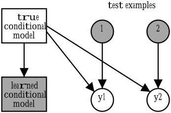
Given the assumption that the training and test data are independent, we are proposing to predict test labels by building a graph, asserting joint potentials over pairs of labels (from a learned coordination classifier), and using belief propagation to make dependent predictions. Why does it make sense to make dependent predictions of iid labels? It turns out that this approach is justified even when taking the independence assumptions into account. Figure 1 illustrates the basic argument. In a standard machine learning setting, it is indeed true that, given the correct model for generating iid data, the label y1 for an input pattern x1 is independent of the label y2 for another pattern x2. However, note that this requires knowledge of the correct model (or at least its correct structure), which is rarely the case in classification learning. Instead, given only an estimate of the true model obtained from training data, y1 and y2 remain dependent, as Figure 1 clearly shows. That is, in the context of supervised learning it is generally the case that test labels are dependent given a learned model. In fact, it is obvious that supervised learning algorithms correlate the labels on the training data. Our observation is simply that the same principle can also be applied to test data.
Although using a relational technique for an iid problem might still appear awkward, it has a well known precedent in machine learning research: transductive learning [Vapnik, 1998; Zhu et al., 2003]. In transduction, the learner knows the set of test patterns beforehand, and exploits this knowledge to make predictions that are ultimately dependent. In fact, this idea has been exploited in recent approaches to semisupervised learning using Markov random fields [Zhu et al., 2003]. What we are proposing is a general framework for extending standard probabilistic learning algorithms to be transductive in a similar fashion.
Our method can be further motivated by noting that it is a natural extension of standard ideas in supervised iid classification. As observed, learning a coordination classifier P(yiyj|xixj, φ) is a natural generalization of learning methods that use a similarity measure k(xi, xj) to classify test examples x∗i based on similarities k(x∗i , x1), ..., k(x∗i , xn) to the training patterns. In fact, this corresponds to our graph choice (i) above, which only connects test labels to training labels. Coordination classification extends the standard similarity based approach by first learning how patterns predict dependencies between the labels (using standard methods applied in a novel way), and then correlating test predictions over a graph. Although there has indeed been recent work on learning kernels for classification [Lanckriet et al., 2004], as well as transductive learning with kernels [Xu et al., 2004], thus far these formulations have remained hard to extend and apply in practice.
Another interesting view of coordination classification is that it is a novel form of ensemble method. That is, the label for a test pattern x∗i is computed by a combination of votes from multiple predictors associated with different test (and training) patterns x(∗) j . In fact, even remotely connected patterns can influence a classification via belief propagation.
As an ensemble method, coordination classification has some useful features. First, it only requires the training of a single base classifier P(yiyj|xixj, φ), rather than multiple base classifiers trained from perturbed data. Second, as with boosting and bagging, coordination classification increases the representational capacity of an original (univariate) classifier. That is, given a classifier representation for a single label P(yi|xi, θ), as mentioned previously, a coordination classifier P (yiyj |xixj , φ) doubles the number of input features and squares the number of output classes. In addition, the prediction of a test label can, in principle, depend on all training and test patterns. Of course, simply increasing the representational capacity of a base classifier increases the risk of overfitting. However, the advantage of ensemble methods is that the resulting classifier, although more complex, is "smoothed" by a principled form of model combination, which helps avoid overfitting while exploiting added representational complexity. That is, the process of model combination can be used to reduce the variance of the learned predictor. In our case, we base our model combination principle on inference in a Markov random field. We will see below that, in fact, coordination classification is competitive as an ensemble technique.
The biggest drawback of coordination classification is the need to perform probabilistic inference (via loopy belief propagation) in order to label test instances. However, we have still found the method to be robust to approximations, like running only a single iteration of loopy belief propagation, or even just taking local votes or products.
4 Experimental Results
We implemented the proposed coordination classification technique for a few different forms of probabilistic classifiers and using various standard iid data sets. Our intent was to determine whether the approach indeed had merit and was also robust to alterations in classifiers and data sets. Our experiments were conducted on standard two-class benchmark data sets from the UCI repository. The data sets used were: 1. australian, 2. breast, 3. chess, 4. cleve, 5. corral, 6. crx, 7. diabetes, 8. flare, 9. german, 10. glass2, 11. heart, 12. hepatitis, 13. mofn-3-7, 14. pima, and 15. vote. All of our experimental results were obtained by 5-fold cross validation, repeated 10 times for different randomizations of the graph structures. The tables and plots report averages of these results, with standard deviations included in the tables.
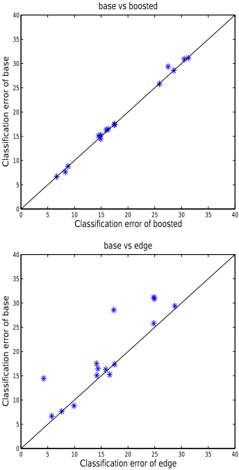
Table 1 and Figure 2 show the results of our first experiment. In this case, we implemented a standard logistic regression model, using unaltered input features, to learn a base coordination classifier P(yiyj|xixj, φ). Classification was performed by running loopy belief propagation until the test labels stabilized (usually after 2 to 8 iterations). In the first experiment we used a graph over test labels only, to determine whether introducing label dependency would have any beneficial effect (see "edge" results). Here we subsampled test-test edges uniformly at random for an overall density of 18 edges per test example. Table 1 and Figure 2 show the resulting misclassification error obtained by coordination classification in comparison to learning a standard logistic regression model, P(yi|xi, θ). Here we see a notable reduction in overall misclassification error (19%→16%), with a significant improvement on some data sets (Breast, -10%, Diabetes, -6%, MofN, -11%, Pima, -6%), and a minor increase on two data sets (Cleve, +1%, and Corral, +1%).
Table 1 also compares the error of coordination classification to boosting the base logistic regression model P(yi|xi, θ). Here we used 18 rounds of Adaboost [Freund and Schapire, 1996; 1997], thereby combining approximately the same number of votes per test pattern as coordination classification. This experiment shows that as an ensemble method, coordination classification performs competitively in this case. An advantage of coordination classification is that it only needs to learn a single base classifier, as opposed to the multiple training episodes required by boosting. The need to run loopy belief propagation on the output labels is a disadvantage however.
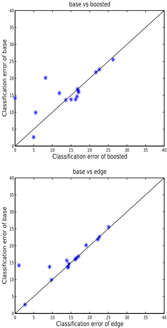
To investigate the robustness of the method, we repeated the previous experiments using a different base classifier. Table 2 and Figure 3 show the results of an experiment using naive Bayes instead of logistic regression as the base classification method. Here the results are not as strong as the first case we tried, although they are still credible. Note that boosting obtains a few larger improvements, but also larger losses. Classification coordination appears to be fairly stable.
| base | boosted | ∆± std | edge | ∆± std | |
|---|---|---|---|---|---|
| australian | 15.1 | 14.5 | -0.6± 0.4 | 14.2 | -0.9± 0.9 |
| breast | 14.5 | 14.9 | 0.4± 0.3 | 4.2 | -10.3± 2.4 |
| chess | 7.6 | 8.3 | 0.7± 0.2 | 7.6 | 0± 0.1 |
| cleve | 15.3 | 14.9 | -0.4± 0.6 | 16.6 | 1.3± 1.1 |
| corral | 8.8 | 8.8 | 0± 0.0 | 9.9 | 1.1± 0.9 |
| crx | 16.5 | 16.3 | -0.2± 0.4 | 14.4 | -2.1± 0.8 |
| diabetes | 31.2 | 31.3 | 0.1± 0.1 | 24.8 | -6.4± 1.1 |
| flare | 17.4 | 17.5 | 0.1± 0.5 | 17.5 | 0.1± 1.3 |
| german | 25.8 | 25.9 | 0.1± 0.1 | 24.8 | -1.0± 1.0 |
| glass2 | 29.4 | 27.5 | -1.9± 1.3 | 28.8 | -0.6± 4.7 |
| heart | 16.3 | 15.9 | -0.4± 0.4 | 15.9 | -0.4± 1.9 |
| hepatitis | 17.5 | 17.5 | 0± 0.0 | 14.1 | -3.4± 3.0 |
| mofn-3-7 | 28.6 | 28.6 | 0± 0.0 | 17.3 | -11.3± 0.8 |
| pima | 30.9 | 30.5 | -0.4± 0.3 | 24.9 | -6.0± 0.8 |
| vote | 6.7 | 6.7 | 0± 0.8 | 5.8 | -0.9± 0.8 |
| average | 18.8 | 18.6 | -0.2± 0.4 | 16.1 | -2.7± 1.4 |
| base | boosted | ∆± std | edge | ∆± std | |
|---|---|---|---|---|---|
| australian | 13.8 | 16.2 | 2.4± 1.6 | 14.2 | 0.4± 0.4 |
| breast | 2.6 | 5.0 | 2.4± 1.1 | 2.7 | 0.1± 0.1 |
| chess | 20.1 | 8.2 | -11.9± 3.1 | 19.1 | -1.0± 0.6 |
| cleve | 16.3 | 17.0 | 0.7± 0.4 | 16.4 | 0.1± 0.2 |
| corral | 13.6 | 13.6 | 0± 5.5 | 14.2 | 0.6± 0.7 |
| crx | 14.6 | 16.6 | 2.0± 0.9 | 14.4 | -0.2± 0.2 |
| diabetes | 22.6 | 22.6 | 0± 0.0 | 22.6 | 0± 0.2 |
| flare | 16.8 | 16.7 | -0.1± 0.1 | 17.0 | 0.2± 0.4 |
| german | 25.5 | 26.3 | 0.8± 0.7 | 25.1 | -0.4± 0.6 |
| glass2 | 15.6 | 11.9 | -3.7± 1.2 | 13.9 | -1.7± 1.2 |
| heart | 15.9 | 17.0 | 1.1± 1.3 | 16.1 | 0.2± 0.2 |
| hepatitis | 13.8 | 15.0 | 1.2± 6.1 | 9.3 | -4.5± 1.2 |
| mofn-3-7 | 14.2 | 0.0 | -14.2± 0.6 | 1.0 | -13.2± 0.8 |
| pima | 21.8 | 21.7 | -0.1± 0.1 | 22.2 | 0.4± 0.4 |
| vote | 9.9 | 5.5 | -4.4± 1.8 | 9.8 | -0.1± 0.2 |
| average | 15.8 | 14.2 | -1.6± 1.6 | 14.5 | -1.3± 0.5 |
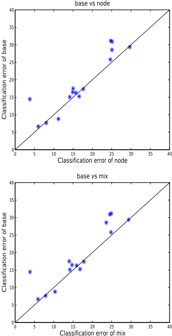
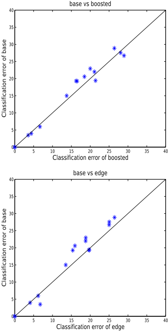
The above experiments were run using only edges between test labels. To compare to standard approaches for iid data, we repeated the experiments using only edges between test and training labels, hence decoupling the test labels and eliminating the need for belief propagation (as discussed in Section 2.2). In this case, test labels are predicted independently. Table 3 and Figure 4 (top) still show, however, that this approach generally improves the base logistic regression classifier P(yi|xi, θ) (see "node" results). We conclude that correlating the test labels appears to be a beneficial idea, even in an iid setting. The marginal improvement of label dependence, although positive, might be secondary to the benefit of learning a similarity measure.
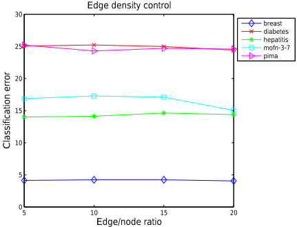
All of the previous results were obtained by subsampling edges at a density of 18 edges per test label. To test the sensitivity of our results to the edge density, we repeated the first experiment (test-test edges) using different edge densities. Figure 5 shows that the performance of coordination classification does not appear to be sensitive to edge density.
Finally, we experimented with the combined edge approach (iii) which randomly mixed test-test edges and testtrain edges yielding the results of Table 3 and Figure 4 (bottom). The results in this case do not appear to surpass the performance of using test only edges (see "mix" results).
5 Extensions
All of our results so far have involved probabilistic classifiers whose output is a conditional distribution over the label y given the input pattern x. Of course, many of the most important classification learning technologies, such as decision trees and support vector machines do not naturally produce probabilistic classifications over the class label (although they can be extended in various ways to do this [Platt, 2000]). This raises the obvious question of generalizing our technique to consider nonprobabilistic classifiers.
It is always possible to extend a classification learning method to learn to predict label pairs (yi, yj) given paired input patterns (xi, xj). The difficulty is combining several paired predictions to render a sensible classification for a single test pattern. A convenient way to do this would be to convert the predicted outputs to nonnegative potentials over labelings. However, rather than do this, we tried the simpler alternative of combining pair classifications by a simple vote to classify a single test pattern x∗i . This is a less powerful combination method than loopy belief propagation, but requires fewer extensions to existing methods to test the coordination classifier idea in these cases.
To test this simple idea, we conducted an experiment on the same UCI data using a neural network classifier. Specifically we used a feedforward neural network with one hidden layer and logistic activation functions. The base neural network used one output unit, whereas the pairwise neural network used four output units (two units to indicate the class of each of the two input vectors) and double the number of input units. In each case the number of hidden units was set to 20, subject to the constraint that (nin + nout) × nhidden ≤ train size/2. We trained the networks to minimize cross entropy error using the quasi-Newton method from Netlab
| base | node | ∆± std | mix | ∆± std | |
|---|---|---|---|---|---|
| australian | 15.1 | 14.1 | -1.0± 0.9 | 14.2 | -0.9± 0.9 |
| breast | 14.5 | 3.8 | -10.7± 2.4 | 3.8 | -10.7± 2.5 |
| chess | 7.6 | 8.1 | 0.5± 0.3 | 7.9 | 0.3± 0.2 |
| cleve | 15.3 | 16.6 | 1.3± 1.3 | 16.8 | 1.5± 1.4 |
| corral | 8.8 | 11.2 | 2.4± 1.2 | 10.3 | 1.5± 0.8 |
| crx | 16.5 | 14.9 | -1.6± 0.8 | 14.7 | -1.8± 0.9 |
| diabetes | 31.2 | 24.7 | -6.5± 1.3 | 24.9 | -6.3± 1.3 |
| flare | 17.4 | 17.6 | 0.2± 1.2 | 17.8 | 0.4± 1.1 |
| german | 25.8 | 24.7 | -1.1± 0.9 | 24.8 | -1.0± 0.9 |
| glass2 | 29.4 | 29.7 | 0.3± 5.0 | 29.4 | 0± 4.6 |
| heart | 16.3 | 15.7 | -0.6± 2.0 | 15.9 | -0.4± 1.8 |
| hepatitis | 17.5 | 15.0 | -2.5± 3.4 | 14.0 | -3.5± 2.8 |
| mofn-3-7 | 28.6 | 25.1 | -3.5± 0.2 | 23.6 | -5.0± 0.4 |
| pima | 30.9 | 25.1 | -5.8± 0.8 | 24.5 | -6.4± 1.0 |
| vote | 6.7 | 6.0 | -0.7± 0.8 | 5.9 | -0.8± 0.7 |
| average | 18.8 | 16.8 | -2.0± 1.5 | 16.6 | -2.2± 1.4 |
[Nabney, 2001] (www.ncrg.aston.ac.uk/netlab).
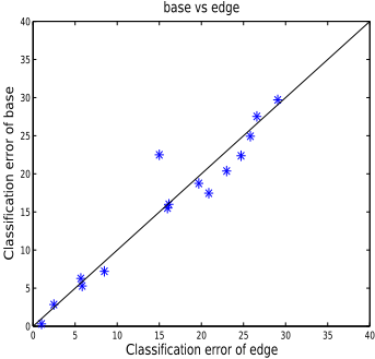
Once a pairwise neural network classifier was learned, we classified test examples according to the previous "edge" model, again by building a random graph between test labels (using an average of 18 edges per test label as before), using the learned coordination neural network to make hard predictions for each edge, and then combining the edge predictions using a simple vote to classify each test example. Table 4 ("edge") and Figure 6 show the results of this experiment. Surprisingly, we still obtain a slight overall reduction in misclassification error over the base level neural network classifier, while again competing well against boosting.
Although encouraging, our results are not as positive in every case. We also conducted a simple experiment with decision trees [Quinlan, 1993] as the base coordination classifier, once again combining these predictions with a simple vote to label specific test patterns. Unfortunately, we did not observe an overall improvement over the base decision tree classifier in this case; see Figure 7. This result suggests that a more powerful model combination idea might be required to achieve robust improvements more generally.
6 Conclusion
We have proposed a novel classification learning strategy that coordinates the prediction of test labels on a graph over the data. The coordination classification idea can be used to extend any probabilistic classification approach quite naturally, and even seems to be applicable to nonprobabilistic techniques as well (although more research needs to be done).
One insight behind the technique is that making correlated predictions of test labels is justified, even advantageous, in the standard iid setting. This fact has often been overlooked in classification learning, therefore we believe it to be a point worth emphasizing. The ability to learn and predict coordinated test labels, combining them with probabilistic inference, provides a flexible new tool for improving classification accuracy on iid data.
| base | boosted | ∆± std | edge | ∆± std | |
|---|---|---|---|---|---|
| australian | 19.3 | 16.5 | -2.8± 0.7 | 15.4 | -3.9± 0.4 |
| breast | 4.0 | 4.4 | 0.4± 0.6 | 4.1 | 0.1± 0.4 |
| chess | 3.5 | 3.6 | 0.1± 0.2 | 6.7 | 3.2± 0.9 |
| cleve | 22.9 | 20.0 | -2.9± 1.4 | 18.8 | -4.1± 1.3 |
| corral | 0 | 0 | 0± 0.0 | 0 | 0± 0.0 |
| crx | 20.6 | 18.5 | -2.1± 0.9 | 15.9 | -4.7± 1.9 |
| diabetes | 27.6 | 28.1 | 0.5± 0.8 | 25.0 | -2.6± 0.9 |
| flare | 19.4 | 21.4 | 2.0± 0.5 | 19.7 | 0.3± 0.4 |
| german | 28.9 | 26.4 | -2.5± 0.6 | 26.4 | -2.5± 1.0 |
| glass2 | 19.3 | 16.3 | -3.0± 1.5 | 19.8 | 0.5± 1.2 |
| heart | 22.0 | 21.1 | -0.9± 2.1 | 18.8 | -3.2± 1.0 |
| hepatitis | 15.0 | 13.8 | -1.2± 3.5 | 13.5 | -1.5± 2.0 |
| mofn-3-7 | 0 | 0 | 0± 0.0 | 0 | 0± 0.0 |
| pima | 26.7 | 29.0 | 2.3± 0.8 | 25.0 | -1.7± 0.6 |
| vote | 6.0 | 6.7 | 0.7± 0.9 | 6.2 | 0.2± 0.4 |
| average | 15.7 | 15.0 | -0.7± 1.0 | 14.4 | -1.3± 0.8 |
One idea for future work that we are considering is to extend the notion of a pairwise edge classifier to a more general clique classifier. We are also investigating alternative principles for defining potentials on label pairs to see perhaps if there are other combination ideas that work more effectively. Finally, we are also investigating whether combining standard "single node" classifiers with our generalized "edge" predictors might lead to further accuracy improvements.
Acknowledgments
Research supported by the Alberta Ingenuity Centre for Machine Learning, NSERC, MITACS, and the Canada Research Chairs program.
@inproceedings{ijcai2005p216,
  title     = {Learning Coordination Classifiers},
  author    = {Guo, Yuhong and Greiner, Russell and Schuurmans, Dale},
  booktitle = {Proceedings of the Nineteenth International Joint Conference on
               Artificial Intelligence, {IJCAI-05}},
  publisher = {International Joint Conferences on Artificial Intelligence},
  editor    = {Leslie Pack Kaelbling and Alessandro Saffiotti},
  pages     = {714--720},
  year      = {2005},
  url       = {https://ijcai.org/proceedings/2005/216},
}
TY - CPAPER TI - Learning Coordination Classifiers AU - Guo, Yuhong AU - Greiner, Russell AU - Schuurmans, Dale T2 - Proceedings of the Nineteenth International Joint Conference on Artificial Intelligence, IJCAI-05 PB - International Joint Conferences on Artificial Intelligence PY - 2005 SP - 714 EP - 720 UR - https://ijcai.org/proceedings/2005/216 ER -Copied
Machine-readable versions of this paper, for tools and AI agents:





