Optimal Nonmyopic Value of Information in Graphical Models - Efficient Algorithms and Theoretical Limits

1 Introduction

In probabilistic reasoning, where one can choose among several possible but expensive observations, it is often a central issue to decide which variables to observe in order to most effectively increase the expected utility. In a medical expert system [14], for example, multiple tests are available, and each test has a different cost. In such systems, it is thus important to decide which tests to perform in order to become most certain about the patient's condition, at a minimum cost. Occasionally, the cost of testing can even exceed the value of information for any possible outcome.

The following running example motivates our research and is empirically evaluated in Section 7. Consider a temperature monitoring task, where wireless temperature sensors are distributed across a building. The task is to become most certain about the temperature distribution, whilst minimizing energy expenditure, a critically constrained resource [4].

Many researchers have suggested the use of myopic (greedy) approaches to select observations [13; 15; 5; 1]. Unfortunately, this heuristic does not provide any performance guarantees. In this paper, we present efficient algorithms, which guarantee optimal nonmyopic value of information in chain graphical models such as Hidden Markov Models (HMMs). We address two settings: subset selection, where the optimal subset of observations is obtained in an open-loop fashion, and conditional plans, a closed-loop plan where the observation strategy depends on the actual value of the observed variables (c.f. Fig. 1(a)). To our knowledge, these are the first optimal and efficient algorithms for these tasks for this class of graphical models. For both settings, we address the filtering and the smoothing versions: Filtering is important in online decision making, where our decisions can only utilize observations made in the past. Smoothing arises for example in structured classification tasks, where there is no temporal dimension in the data, and hence all observations can be taken into account. We evaluate our algorithms empirically on three real-world datasets, and also show that they are well-suited for interactive classification of sequential data.

Most problems in graphical models, such as probabilistic inference and the most probable explanation, that can be solved efficiently for chain-structured graphs, can also be solved efficiently for polytrees. We prove that the problem of maximizing value of information is NPPP-hard even for discrete polytree graphical models, giving a complexity theoretic classification of a core artificial intelligence problem. NPPP-hard problems are believed to be significantly harder than NP-complete or even #P-complete problems commonly arising in the context of graphical models. As a special case, we also prove that computing conditional entropies is #P-complete even in the case of discrete polytrees. This is a surprising result about a measure of uncertainty that is frequently used in practice.

2 Optimization criteria

In order to maximize value of information, our objective functions should depend on probability distributions over variables. Let S = {X1, . . . ,Xn} be a set of discrete random variables. We consider a class of local reward functions R, which are defined on the marginal probability distributions of the variables. This class has the computational advantage that local rewards can be evaluated using probabilistic inference techniques. The total reward will then be the sum of all local rewards.

Let O be a subset of S. Then P(Xj | O = o) denotes the marginal distribution of variable Xj conditioned on observations o. For classification purposes, it can be more appropriate to consider the max-marginals P max (Xj = xj | O = o) = maxx P(X = x,Xj = xj | O = o), that is, for Xj set to value xj , the probability of the most probable assignment to all other random variables conditioned on the observations o. The local reward Rj is a functional on the probability distribution P or P max over Xj . We write

as an abbreviation to indicate expected local rewards, where the expectation is taken over all assignments o to the observations O. Important measures for value of information include:

• Entropy. If we set Rj(P(Xj | O)) = -H(Xj | O) = ∑xj,o P(xj, o) logP(xj | o), the objective in the optimization problem becomes to minimize the sum of residual entropies. We choose this reward function in our running example to measure the uncertainty about the temperature distribution.
• Maximum expected utility. The concept of local reward functions also includes the concept of utility nodes in influence diagrams. If Uj : Aj × domXj → R is a utility function mapping an action a ∈ Aj and an outcome x ∈ domXj to a reward, then the maximum expected utility principle states that actions should be selected as to maximize EUj(a | o) = ∑x P(x | o)Uj(a, x). The more certain we are about Xj, the more economically we can choose our action. Hence we can define our local reward function R(P(Xj | O)) = ∑o P(o)maxa EUj(a | o).
• Margin. We can also consider the margin of confidence: Rj(P max (Xj | O)) = ∑o P(o)[P max (x∗j | o)-P max (¯xj | o)], where x∗ = argmaxxj P max (xj | o) and ¯x = argmaxxj̸=x∗ P max (xj | o), which describes the margin between the most likely outcome and the closest runner up. This reward function is very useful for structured classification purposes, as shown in Sec. 7.

These examples demonstrate the generality of our notion of local reward. One can generalize the algorithms even more, e.g., to measure the total entropy or the margin between the most probable explanation and its runner up. Details are omitted here due to space limitations.

We also want to capture the constraint that observations are expensive. This can mean that each observation Xj has an associated positive penalty Cj that effectively decreases the reward. In our example, we might be interested in trading off accuracy with sensing energy expenditure. Alternatively, it is also possible to define a budget B for selecting observations, where each one is associated with an integer cost βj. Here, we want to select observations whose sum cost is within the budget, but these costs do not decrease the reward. In our running example, the sensors could be powered by solar power, and regain a certain amount of energy per day, which allows a certain amount of sensing. Our formulation of the optimization problems allows both for penalties and budgets. To simplify notation we also write C(O) = ∑Xj∈O Cj and β(O) = ∑Xj∈O βj to extend C and β to sets.

3 Decomposing Rewards

In the following Sections 4 and 5, we present efficient algorithms for two problems of optimizing value of information in the class of chain graphical models.

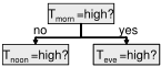
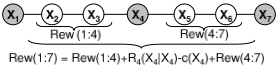
Figure 1: Example, and decomposing reward idea

The set of random variables S = {X1, . . . ,Xn} forms a chain graphical model (a chain), if Xi is conditionally independent of Xk given Xj whenever i < j < k. We can assume that the joint distribution is specified by the prior P(X1) and conditional probability distributions P(Xi+1 | Xi). The time series model for the temperature measured by one sensor in our example can be formulated as a chain graphical model.

Chain graphical models originating from time series have additional, specific properties: In a system for online decision making, only observations from the past and present time steps can be taken into account, not observations which will be made in the future. This is in general referred to as the filtering problem. In this setting, the notation P(Xi | O) will refer to the distribution of Xi conditional on observations in O prior to and including time i. For structured classification problems as discussed in Section 7, in general observations made anywhere in the chain must be taken into account. This situation is usually referred to as the smoothing problem. We will provide algorithms both for filtering and smoothing.

We will now describe the key insight, which allows for efficient optimization in chains. Consider a set of observations O ⊆ S. If the j variable is observed, i.e., Xj ∈ O, then the local reward is simply R(Xj | O) = R(Xj | Xj). Now consider Xj /∈ O, and let Oj be the subset of O containing the closest ancestor (and for the smoothing problem also the closest descendant) of Xj in O. The conditional independence property of the graphical model implies that, given Oj, Xj is independent of the rest of the observed variables, i.e., P(Xj | O) = P(Xj | Oj). Thus, it follows that R(Xj | O) = R(Xj | Oj).

These observations imply that the expected reward of some set of observations decomposes along the chain. For simplicity of notation, we add two independent dummy variables X0 and Xn+1, where R0 = C0 = β0 = Rn+1 = Cn+1 = βn+1 = 0. Let O = {Xi0 , . . . ,Xim+1 } where il < il+1, i0 = 0 and im+1 = n + 1. Using this notation, the total reward R(O) = ∑j Rj(Xj | O) for the smoothing case is given by:

In filtering settings, we simply replace Rj(Xj | Xiv ,Xiv+1 ) by Rj(Xj | Xiv ). Figure 1(b) illustrates this decomposition.

Consider now a Hidden Markov Model unrolled for n time steps, i.e., S can be partitioned into the hidden variables {X1, . . . ,Xn} and the emission variables {Y1, . . . , Yn}. In HMMs, the Yi are observed and the variables Xi form a chain. In many applications, some of which are discussed in Section 7, we can observe some of the hidden variables, e.g., by asking an expert, in addition to observing the emission variables. In these cases, the problem of selecting expert labels also belongs to the class of chain graphical models addressed by this paper.

4 Subset Selection

In the subset selection problem, we want to find a most informative subset of the variables to observe in advance, i.e., before any observations are made. In our running example, we would, before deploying the sensors, identify k time points that are expected to provide the most informative sensor readings according to our model.

First, define the objective function L on subsets of S by

The subset selection problem is to find the optimal subset

maximizing the sum of expected local rewards minus the penalties, subject to the constraint that the total cost must not exceed the budget B.

We solve this optimization problem using a dynamic programming algorithm, where the chain is broken into sub-chains using the insight from Sec. 3. Consider a sub-chain from variable Xa to Xb. We define La:b(k) to represent the expected total reward for the sub-chain Xa, . . . ,Xb, where Xa (and Xb in the smoothing case) is observed, and with a budget level of k. More formally:

for the filtering version, and

for the smoothing version. Note that L0:n+1(B) = maxO:β(O)≤B L(O), as in Eq. (4.1), i.e., by computing the values for La:b(k), we compute the maximum expected total reward for the entire chain.

We can compute La:b(k) using dynamic programming. The base case is simply:

for filtering, and

for smoothing. The recursion for La:b(k) has two cases: we can choose not to spend any more of the budget, reaching the base case, or we can break the chain into two sub-chains, selecting the optimal observation Xj , where a < j < b:

At first, it may seem that this recursion should consider the optimal split of the budget between the two sub-chains. However,

Input: Budget B, rewards Rj, costs βj and penalties Cj Output: Optimal selection O of observation times begin for 0 ≤ a < b ≤ n+1 do compute La:b(0); for k = 1 to B do for 0 ≤ a < b ≤ n + 1 do sel(-1) := La:b(0); for j = a+1 to b -1 do sel(j) := -Cj +Rj(Xj | Xj) +La:j(0) +Lj:b(k -βj); La:b(k) = maxa<j<b sel(j); Λa:b(k) = argmaxa<j<b sel(j); end end a := 0; b := n + 1; k := B; O := ∅; repeat j := Λa:b(k); if j ≥ 0 then O := O ∪ {Xj}; k := k - βj ; until j = -1; end

since the subset problem is open-loop and the order of the observations is irrelevant, we only need to consider split points where the first sub-chain receives zero budget.

A pseudo code implementation is given in Alg. 1. If we do not consider different costs β, we would simply choose βj = 1 for all variables and compute La:b(N). Alg. 1 uses the quantities Λa:b to recover the optimal subset by tracing the maximal values occurring in the dynamic programming equations. Using an induction proof, we obtain:

Theorem 1. The dynamic programming algorithm described above computes the optimal subset with budget B in ( 1 6 n3 + O(n2 ))B evaluations of expected local rewards.

If the variables Xi are continuous, our algorithm is still applicable when the integrations and inferences necessary for computing the expected rewards can be performed efficiently.

5 Conditional Plan

In the conditional plan problem, we want to compute an optimal querying policy: We sequentially observe a variable, pay the penalty, and depending on the observed values, select the next query as long as our budget suffices. The objective is to find the plan with the highest expected reward, where, for each possible sequence of observations, the budget B is not exceeded. For filtering, we can only select observations in the future, whereas in the smoothing case, the next observation can be anywhere in the chain. In our running example, the filtering algorithm would be most appropriate: The sensors would sequentially follow the conditional plan, deciding on the most informative times to sense based on the previous observations. Fig. 1(a) shows an example of such a conditional plan.

The formal definition of the objective function J is given recursively. The base case considers the exhausted budget:

The recursion, J(O = o; k), represents the maximum expected reward of the conditional plan for the chain where O = o has been observed and the budget is limited to k:

The optimal plan has reward J(∅; B).

We propose a dynamic programming algorithm for obtaining the optimal conditional plan that is similar to the subset algorithm presented in Sec. 4. Again, we utilize the decomposition of rewards described in Section 3. The difference here is that the observation selection and budget allocation now depend on the actual values of the observations.

We again consider sub-chains Xa, . . . ,Xb. The base case deals with the zero budget setting:

for filtering, and

for smoothing. The recursion defines Ja:b(xa; k) (Ja:b(xa, xb; k) for smoothing), the expected reward for the problem restricted to the sub-chain Xa, . . . ,Xb conditioned on the values of Xa (and Xb for smoothing), and with budget limited by k. To compute this quantity, we again iterate through possible split points j, such that a < j < b. Here we observe a notable difference between the filtering and the smoothing case. For smoothing, we now must consider all possible splits of the budget between the two resulting sub-chains, since an observation at time j might require us to make an additional, earlier observation:

Looking back in time is not possible in the filtering case, hence the recursion simplifies to

The optimal reward is obtained by J0:n+1(∅;B) = J(∅;B). Alg. 5 presents a pseudo code implementation for the smoothing version - the filtering case is a straight-forward modification. The plan itself is compactly encoded in the quantities πa:b which determines the next variable to query and σa:b, which determines the allocation of the budget. Considering the exponential number of possible sequences of observations, it is remarkable that the optimal plan can even be represented using only polynomial space. Alg. 5 indicates how the computed plan can be executed. The procedure is recursive, requiring the parameters a := 0, xa := 1, b := n + 1, xb := 1 and k := B for the initial call. Again, by induction, we obtain:

Theorem 2. The algorithm for smoothing presented above computes an optimal conditional plan in d3 ·B2 ·( 16 n3+O(n2 )) evaluations of local rewards, where d is the maximum domain size of the random variables X1, . . . ,Xn. In the filtering case, or if no budget is used, the optimal plan can be computed using d3 · B · ( 1 6 n3 +O(n2 )) or d3 · ( 1 6 n4 +O(n3 )) evaluations respectively.

The faster computation for the no budget case is obtained by observing that we do not require the third maximum computation, which distributes the budget into the sub-chains.

Input: Budget B, rewards Rj, costs βj and penalties Cj Output: Optimal conditional plan (πa:b, σa:b) begin for 0 ≤a < b≤ n + 1, xa ∈ domXa, xb ∈ domXb do compute Ja:b(xa, xb; 0); for k = 1 to B do for 0≤a<b≤n+1, xa ∈domXa, xb ∈domXb do sel(-1) := Ja:b(0); for a < j < b do sel(j) := -Cj +Rj(Xj | Xj); for a < j < b, xj ∈ domXj do for 0 ≤ l ≤ k -βj do ; bd(l) := Ja:j (xa, xj ; l) + Jj:b(xj , xb; k - l - βj ); sel(j) := sel(j) +P(xj | xa, xb) · maxl bd(j); σ(j, xj) = argmaxl bd(j); end Ja:b(k) = maxa<j<b sel(j); πa:b(xa, xb; k) = argmaxa<j<b sel(j); for xj ∈ domXπa:b(k) do σa:b(xa, xb, xj ; k) = σ(πa:b(k), xj ); end end end

Input: Budget k, observations Xa = xa, Xb = xb, σ, π begin j := πa:b(xa, xb; k); if j ≥ 0 then Observe Xj = xj ; l := σa:b(xa, xb, xj; k); Recurse with k := l, a := a, b := j; Recurse with k := k - l - βj , a := j, b := b; end end

6 Theoretical Limits

Many problems that can be solved efficiently for discrete chain graphical models can also be efficiently solved for discrete polytrees. Examples include probabilistic inference and the most probable explanation (MPE). Surprisingly, we prove that for the optimization problems discussed in this paper, this generalization is not possible, unless P = NP. All proofs in this section are stated in the Appendix.

In order to solve the optimization problems, we will most likely have to evaluate the objective function, i.e., the expected local rewards. Our first result states that this problem is intractable even for discrete polytrees.

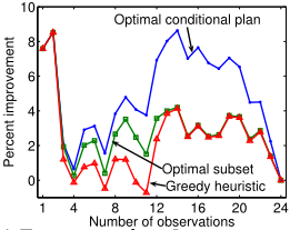
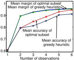
Figure 2: Experimental results.

Theorem 3. The computation of expected local rewards for discrete polytrees is #P-complete. 1

This negative result can be specialized to the conditional entropy, one of the most frequently used reward function to characterize the residual uncertainty in value of information problems.

Corollary 4. The computation of conditional entropy for discrete polytrees is #P-complete.

Since evaluating local rewards is #P-complete, it can be suspected that the subset selection problem is at least #Phard. We show that it is even NPPP-complete 2 , a complexity class containing problems that are believed to be significantly harder than NP or #P complete problems. This result provides a complexity theoretic classification of value of information, a core AI problem.

Theorem5. Subset Selection isNPPP-complete even for discrete polytrees.

For our running example, this implies that the generalized problem of optimally selecting k sensors from a network of correlated sensors is most likely computationally intractable without resorting to heuristics. A corollary extends the hardness of subset selection to the hardness of conditional plans.

Corollary 6. Computing conditional plans is NPPP-hard even for discrete polytrees.

7 Experiments

In this section, we evaluate the proposed methods for several real world data sets. A special focus is on the comparison of the optimal methods with the greedy heuristic and other heuristic methods for selecting observations, and on how the algorithms can be used for interactive structured classification.

7.1 Temperature time series

The first data set consists of temperature time series collected from a sensor network deployed at Intel Research Berkeley [4] as described in our running example. Data was continuously collected for 19 days, linear interpolation was used in case of missing samples. The temperature was measured once every

1#P contains problems such as counting the number of satisfying assignments to a Boolean formula.

2NPPP is natural for AI planning problems [9]. A complete problem is EMAJSAT , where one has to find an assignment to the first k variables of a 3CNF formula, such that the formula is satisfied under the majority of assignments to the remaining variables.

60 minutes, and it was discretized into 10 bins of 2 degrees Kelvin. To avoid overfitting, we used pseudo counts α = 0.5 when learning the model. Using parameter sharing, we learned four sets of transition probabilities: from 12 am - 7am, 7 am - 12 pm, 12 pm - 7 pm and 7 pm - 12 am. Combining the data from three adjacent sensors, we got 53 sample time series.

The goal of this task was to select k out of 24 time points during the day, during which sensor readings are most informative. The experiment was designed to compare the performance of the optimal algorithms, the greedy heuristic, and a uniform spacing heuristic, which distributed the k observations uniformly over the day. Fig. 2(a) shows the relative improvement of the optimal algorithms and the greedy heuristic over the uniform spacing heuristic. The performance is measured in decrease of expected entropy, with zero observations as the baseline. It can be seen that if k is less than about the half of all possible observations, the optimal algorithms decreased the expected uncertainty by several percent over both heuristics. The improvement gained by the optimal plan over the subset selection algorithms appears to become more drastic if a large number of observations (over half of all possible observations) is allowed. Furthermore, for a large number of observations, the optimal subset and the subset selected by the greedy heuristic were almost identical.

7.2 CpG-Island detection

We then studied the bioinformatics problem of finding CpG islands in DNA sequences. CpG islands are regions in the genome with a high concentration of the cytosine-guanine sequence. These areas are believed to be mainly located around the promoters of genes, which are frequently expressed in the cell. In our experiment, we considered the gene loci HS381K22, AF047825 and AL133174, for which the GenBank annotation listed three, two and one CpG islands each. We ran our algorithm on a 50 base window at the beginning and end of each island, using the transition and emission probabilities from [6] for our Hidden Markov Model, and we used the sum of margins as reward function.

The goal of this experiment was to locate the beginning and ending of the CpG islands more precisely by asking experts, whether or not certain bases belong to the CpG region or not. Fig. 2(b) shows the mean classification accuracy and mean margin scores for an increasing number of observations. The results indicate that, although the expected margin scores are similar for the optimal algorithm and the greedy heuristic, the mean classification performance of the optimal algorithm was still better than the performance of the greedy heuristic.

7.3 Part-of-Speech Tagging

In our third experiment, we investigated the structured classification task of part-of-speech (POS) tagging [3]. Problem instances are sequences of words (sentences), where each word is part of an entity (e.g., "United States of America"), and each entity belongs to one of five categories: Location, Miscellaneous, Organization, Person or Other. Imagine an application, where automatic information extraction is guided by an expert: Our algorithms compute an optimal conditional plan for asking the expert, trying to optimize classification performance while requiring as little expert interaction as possible.

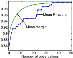
We used a conditional random field for the structured classification task, where each node corresponds to a word, and the joint distribution is described by node potentials and edge potentials. The sum of margins was used as reward function. Measure of classification performance was the F1 score, the geometric mean of precision and recall. The goal of this experiment was to analyze how the addition of expert labels increases the classification performance, and how the indirect, decomposing reward function used in our algorithms corresponds to real world classification performance.

Figure 2(c) shows the increase of the mean expected margin and F1 score for an increasing number of observations, summarized over ten 50 word sequences. It can be seen that the classification performance can be effectively enhanced by optimally incorporating expert labels. Requesting only three out of 50 labels increased the mean F1 score from by more than five percent. The following example illustrates this effect: In one scenario both words of an entity, the sportsman 'P. Simmons', were classified incorrectly - 'P.' as Other and 'Simmons' as Miscellaneous. The first request of the optimal conditional plan was to label 'Simmons'. Upon labeling this word correctly, the word 'P.' was automatically labeled correctly also, resulting in an F1 score of 100 percent.

8 RelatedWork

Decision Trees [12] popularized the value of information as a criterion for creating conditional plans. Unfortunately, there are no guarantees on the performance of this greedy method. Bayer-Zubek [1] proposed a heuristic method based on the Markov Decision Process framework. Several researchers [15; 5] suggested myopic, i.e., greedy approaches for selectively gathering evidence in graphical models. Heckerman et al. [7] propose a method to compute the maximum expected utility for specific sets of observations. While their work considers more general graphical models than this paper, they provide only large sample guarantees for the evaluation of a given sequence of observations, and use a heuristic without guarantees to select such sequences The subset selection problem as an instance of feature selection is a central issue in machine learning, with a vast amount of literature (see [10] for a survey). The problem of choosing observations also has a strong connection to the field of active learning [2] in which the learning system designs experiments based on its observations.

9 Conclusions

We have described novel efficient algorithms for optimal subset selection and conditional plan computation in chain graphical models, including HMMs. Empirical evaluation indicates that these algorithms can improve upon commonly used heuristics for decreasing expected uncertainty. Our algorithms can also effectively enhance performance in interactive structured classification tasks.

Unfortunately, the optimization problems become intractable for even a slight generalization of chains. We presented surprising theoretical limits, which indicate that commonly used local reward functions, such as conditional entropies, cannot be efficiently computed even in discrete polytree graphical models. We also identified optimization of value of information as a new class of problems that are intractable (NPPP-complete) for polytrees.

Our hardness results, along with other recent results for polytree graphical models, the NP-completeness of maximum a posteriori assignment [11] and NP-hardness of inference in conditional linear Gaussian models [8], suggest the possibility of developing a generalized complexity characterization of problems that are hard in polytree graphical models.

In light of these theoretical limits for computing optimal solutions, it is a natural question to ask whether approximation algorithms with non-trivial performance guarantees can be found. We are currently focusing our research in this direction.

Acknowledgements. We would like to thank Ben Taskar for providing the part-of-speech tagging model, and Reuters for making their news archive available. We would also like to thank Brigham Anderson and Andrew Moore for helpful comments and discussions.

Appendix

Proof of Theorem 3. Membership in #P is straightforward. To show hardness, we use a construction similar to the one presented in [11] for the maximum a posteriori problem. Let φ be an instance of #3SAT, where we have to count the number of assignments to X1, . . . ,Xn satisfying φ. Let C = {C1, . . . ,Cm} be the set of clauses. Now create a Bayesian network with nodes Ui for each Xi, each with uniform Bernoulli prior. Add variables Y0, which uniformly varies over {1, . . . , m} and Y1, . . . , Yn with CPTs defined the following way:

In this model, Yn = 0 iff U1, . . . ,Un encode a satisfying assignment of φ. Let all nodes have zero reward, except for Yn, which is assigned the following reward:

Since the prior probability of any assignment is 2-n , the expected reward R(Yn | U1, . . . ,Un) is exactly the number of satisfying assignments to φ.

Proof of Corollary 4. We start from the same construction as in the proof of Theorem 3, and add an additional random variable Z after Yn on the chain. Z | Yn is 0 if Yn = 0, and takes uniformly random values in {0, 1} if Yn ̸= 0. Then H(Z | U = u) is 0 if u is a satisfying assignment, and 1 otherwise. Hence H(Z | O) = 1 -K2-n , where K is the number of satisfying assignments to φ.

Proof of Theorem 5. Membership follows from Theorem 3. Let φ be an instance of EMAJSAT , where we have to find an instantiation of X1, . . . ,Xn such that φ(X1, . . . ,X2n) is true for the majority of assignments to Xn+1, . . . ,X2n. Let C = {C1, . . . , Cm} be the set of 3CNF clauses. Create the Bayesian network shown in Fig. 3, with nodes Ui, each having a uniform Bernoulli prior. Add bivariate variables Yi = (seli, pari), 0 ≤ i ≤ 2n, where seli takes values in {0, . . . ,m} and pari is a parity bit. The CPTs for Yi are defined as: sel0 uniformly varies over {1, . . . ,m}, par0 = 0, and for Y1, . . . , Y2n:

where ⊕ denotes the parity (XOR) operator. We now add variables Z T i and Z F i for 1 ≤ i ≤ n and let

where I denotes the uniform distribution. Similarly, let

Intuitively, Z T i = 1 guarantees us that Ui = 1, whereas Z T i = 0 leaves us uncertain about Ui. The case of Z F i is symmetric.

We use the subset selection algorithm to choose the Zis that encode the solution to EMAJSAT. If Z T i is chosen, it will indicate that Xi should set to true, similarly Z F i indicates a false assignment to Xi. The parity function is going to be used to ensure that exactly one of {Z T i ,Z F i } is observed for each i.

We first assign penalties ∞ to all nodes except Z T i ,Z F i for 1 ≤ i ≤ n, and Uj for n + 1 ≤ j ≤ 2n, which are assigned zero penalty. Let all nodes have zero reward, except for Y2n, which is assigned the following reward:

Note that sel2n = 0 with probability 1 iff U1, . . . , U2n encode a satisfying assignment of φ, as in the proof of Theorem 3. Furthermore, we get positive reward only if we are both certain that sel2n = 0, i.e., the chosen observation set must contain a proof that φ is satisfied, and we are certain about par2n. The parity certainty will only occur if we are certain about the assignment U1, . . . ,U2n. It is only possible to infer the value of each Ui with certainty by observing one of Ui, Z T i or Z F i . Since, for i = 1, . . . , n, the cost of observing Ui is ∞, to receive any reward we must observe at least one of Z T i or Z F i . Assume that we compute the optimal subset ˆO for budget 2n, then we can only receive positive reward by observing exactly one of Z T i or Z F i .

We interpret the selection of Z T i and Z F i as an assignment to the first n variables of EMAJSAT. Let ˆR = R(Y2n | ˆO). We claim that φ ∈ EMAJSAT if and only if ˆR > 0.5. First let φ ∈ EMAJSAT , with assignment x1, . . . , xn to the first n variables. Now add Un+1, . . . , U2n to O and add Z T i to O iff xi = 1 and Z F i to O iff xi = 0. This selection guarantees ˆR > 0.5.

Now assume ˆR > 0.5. We call an assignment to U1, . . . ,U2n consistent if for any 1 ≤ i ≤ n, if Z T i ∈ ˆO, then Ui = 1 and if Z F i ∈ ˆO then Ui = 0. For any consistent assignment, the chance that the observations Zi prove the consistency is 2-n . Hence ˆR > 0.5 implies that the majority of all provably consistent assignments satisfy φ and hence φ ∈ EMAJSAT . This proves that subset selection is NPPP complete.

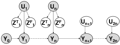
Proof of Corollary 6. The construction in the proof of Theorem 5 also proves that computing conditional plans is NPPPhard, since, in this instance, any plan with positive reward must observe all Un+1, . . . , U2n and one each of the Z1, . . . , Zn, to satisfy the parity condition. In this case, the order of selection is irrelevant, and, hence, the conditional plan effectively performs subset selection.