Minimal and Absent Information in Contexts

1 Introduction

Based on motivational papers by McCarthy [1987] and Giunchiglia [1993] several formalizations of contextual information and inter-contextual information flow have been proposed. Most notable are the propositional logic of context developed by McCarthy, Buvaˇc and Mason [1993; 1998], and the multi-context systems devised by Giunchiglia and Serafini [1994], which later have been associated with the local model semantics introduced by Giunchiglia and Ghidini [2001]. Serafini and Bouquet [2004] have argued from a technical point of view that multi-context systems constitute the most general formal framework. This conclusion is supported by a more conceptual argument of Benerecetti et.al. [2000].

A multi-context system describes the information available in a number of contexts (i.e., to a number of people / agents / databases, etc.) and specifies the information flow between those contexts. The local model semantics defines a system to entail a piece of information, if and only if that piece of information is acquired, independently of how the information flow described by the system is accomplished.

Our first contribution is based on the observation that the local model semantics of a multi-context system is completely determined by the information that is obtained when simulating the information flow specified by the system, in such a way that a minimal amount of information is deduced at each step of the simulation. We define an operator which suitably implements such a simulation, and thus determines the information entailed by the system. This operator constitutes a first constructive account of the local model semantics.

Our second contribution is based on the observation that in multi-context systems, new information is derived based on the presence of other information only. However, in many natural situations (concrete examples will be given below), new information is obtained due to a lack of other information. We propose a generalized framework so as to account for such situations. Non-monotonic reasoning techniques are applied to formulate a suitable semantics for this framework.

We proceed, in section 2, with a brief review of multicontext system syntax and local model semantics. Minimality is discussed in section 3, and the generalized framework is presented in section 4. We conclude, in section 5, with a concise recapitulation of our main observations and results. 1

2 Preliminaries

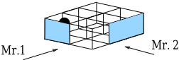
A simple illustration of the main intuitions underlying the multi-context system framework is provided by the situation depicted in figure 1. Two agents, Mr.1 and Mr.2, are looking at a box from different angles. The box is called magic, because neither Mr.1 nor Mr.2 can make out its depth. As some sections of the box are out of sight, both agents have partial information about the box. To express this information, Mr.1 only uses proposition letters l (there is a ball on the left) and r (there is a ball on the right), while Mr.2 also uses a third proposition letter c (there is a ball in the center).

In general, we consider a set of contexts I, and a language Li for each context i ∈ I. We assume I and {Li}i∈I to be fixed, unless specified otherwise. Moreover, for the purpose of this paper we assume each Li to be built over a finite set of proposition letters, using standard propositional connectives.

To state that the information expressed by a formula ϕ ∈ Li is established in context i we use so-called labeled formulas of the form i : ϕ (if no ambiguity arises, we simply refer to labeled formulas as formulas, and we even use capital letters F, G, and H to denote labeled formulas, if the context label is irrelevant). A rule r is an expression of the form:

1 See http://home.student.uva.nl/f.roelofsen/ for all proofs that are omitted or merely sketched here.

where F and all G's are labeled formulas; F is called the consequence of r and is denoted by cons(r); all G's are called premises of r and together make up the set prem(r). Rules without premises are called facts. Rules with at least one premiss are called bridge rules. A multi-context system (system hereafter) is a finite set of rules. A fact describes information that is established in a certain context, independently of which information is obtained in other contexts. A bridge rule specifies which information is obtained in one context, if other pieces of information are acquired in different contexts. Thus a system can be thought of as a specification of contextual information and an inter-contextual information flow.

Example 1 The situation in figure 1 can be modeled by the following system:

1 : ¬r ← 2 : l ← 1 : l ∨ r ← 2 : l ∨ c ∨ r 2 : l ∨ c ∨ r ← 1 : l ∨ r

Mr.1 knows that there is no ball on the right, Mr.2 knows that there is a ball on the left, and if any agent gets to know that there is a ball in the box, then he will inform the other agent.

A classical interpretation m of language Li is called a local model of context i. A set of local models is called a local information state. Intuitively, every local model in a local information state represents a "possible state of affairs". If a local information state contains exactly one local model, then it represents complete information. If it contains more than one local model, then it represents partial information: more than one state of affairs is considered possible. A distributed information state is a set of local information states, one for each context. In conformity with the literature, we will refer to distributed information states as chains.

Example 2 The situation in figure 1, in which Mr.1 knows that there is no ball on the right but does not know whether there is a ball on the left, is represented by a chain whose first component [ {l, ¬r} , {¬l, ¬r} ] contains two local models. As such, the chain reflects Mr.1's uncertainty about the left section of the box.

A chain c satisfies a labeled formula i : ϕ (denoted c |= i : ϕ) iff all local models in its ith component classically satisfy ϕ. A rule r is applicable with respect to a chain c iff c satisfies every premiss of r. Notice that facts are applicable with respect to any chain. A chain c complies with a rule r, iff, whenever r is applicable with respect to c, then c satisfies r's consequence. We call c a solution chain of a system S iff it complies with every rule in S. A formula F is true in S (denoted S |= F ) iff every solution chain of S satisfies F .

Let C denote the set of all chains. Notice that, as each Li is assumed to be built over a finite set of proposition letters, C is assumed to be finite. Let c⊥ denote the chain containing every local model of every context (notice that c⊥ does not satisfy any non-tautological expression); let c⊤ denote the chain containing no local models at all (notice that c⊤ satisfies any expression). If C is a set of chains, then the component-wise union of C is the chain, whose ith component consists of all local models that are in the ith component of some chain in C. If c and c′ are chains, then c \ c′ denotes the chain, whose ith component consists of all local models that are in ci but not in c′i . Finally, we sometimes say that a local model m is (not) in c, when we actually mean that m is (not) in some (any) component ci of c.

3 Minimality

We order chains according to the amount of information they convey. Intuitively, the more local models a chain component contains, the more possibilities it permits, so the less informative it is. Formally, we say that c is less informative than c′ (c ⪯ c′ ), if for every i we have ci ⊇ c′i . If, moreover, for at least one i we have ci ⊃ c′i , then we say that c is strictly less informative than c′ (c ≺ c′ ).

Lemma 1 Let c and c′ be two chains, such that c ⪯ c′ . Then any formula that is satisfied by c is also satisfied by c′ .

We call c minimal among a set of chains C, iff c is in C and no other chain c′ in C is strictly less informative than c. In particular, we call c a minimal solution chain of a system S, if it is minimal among the set of all solution chains of S.

Theorem 1 Every system S has a unique minimal solution chain cS.

Proof. Let CS be the set of all solution chains of S. CS ̸= ∅ as c⊤ ∈ CS for any S. Let cS be the component-wise union of all chains in CS. Then cS ∈ CS and cS ⪯ c for any c ∈ CS. So cS is the unique minimal solution chain of S. □

Theorem 2 The semantics of a system S is completely determined by its unique minimal solution chain cS:

Proof. F is true in S iff F is satisfied by all solution chains of S iff F is satisfied by the component-wise union cS of all solution chains of S. □

Theorem (1) and (2) are extremely useful, because they establish that, to answer queries about a system S, it is no longer necessary to compute all solution chains of S; we only need to consider the system's minimal solution chain cS.

3.1 Computing the Minimal Solution Chain

The minimal solution chain of S can be characterized as the ⪯-least fixpoint of an operator TS, which, intuitively, simulates the information flow specified by S. Let S∗ (c) denote the set of rules in S, which are applicable w.r.t. c. Then we define:

For every rule r in S that is applicable w.r.t. c, TS removes from c all local models that do not satisfy cons(r).

Intuitively, this corresponds to augmenting c with the information expressed by cons(r). In this sense, TS simulates the information flow described by S. As TS(c) is obtained from c only by removing local models from it, TS(c) is always more informative than c.

As (C,⪯) forms a complete lattice, and TS is monotone and continuous w.r.t. ⪯, [Tarski, 1955] yields:

• Theorem 3 TS has a ⪯-least fixpoint, which is obtained after a finite number of consecutive applications of TS to c⊥.

Lemma 2 Let c be a chain and let S be a system. Then c is a fixpoint of TS if and only if c is a solution chain of S.

Theorem 4 Let S be a system. Then the minimal solution chain cS of S coincides with the ⪯-least fixpoint of TS.

From theorems 3 and 4 we conclude that the minimal solution chain cS of a system S is obtained after a finite number of applications of TS to the least informative chain c⊥. But we can even prove a slightly stronger result:

Theorem 5 Let S be a system and let |S| denote the number of bridge rules in S. Then the minimal solution chain cS of S is obtained after at most |S| + 1 applications of TS to c⊥.

In fact, a slightly more involved, but essentially equivalent procedure was introduced for rather different reasons by Roelofsen et.al. [2004]. This procedure was shown to have worst-case time complexity O(|S|2 × 2M ), where M is the maximum number of propositional variables in either one of the contexts involved in S.

Example 3 Consider the system from example 1. Applying TS to c⊥ establishes the facts given by the first two rules of the system. But then Mr.2 knows that there is a ball in the box, so the next application of TS simulates the information flow specified by the third rule of the system: Mr.2 informs Mr.1 of the presence of the ball. The resulting chain is left unaltered by any further application of TS, and therefore constitutes the minimal solution chain of S. The fact that this chain satisfies the formula 1 : l reflects, as desired, that Mr.1 has come to know that there is a ball in the left section of the box.

4 Absent Information

Rules of the form (1) only allow us to model a rather restricted kind of information flow, namely one in which new information is established based on the presence of other information only. There are many natural situations in which information is obtained as a result of the absence of other information. Such situations cannot be modeled by the present formalism.

Example 4 (Coordination) Let d1, d2 be two meteorological databases that collect their respective data from sensors located in different parts of the country. At the end of the day each database produces a weather forecast based on its own data but also on the information obtained by the other database. For example, d1 predicts rain, if that follows from its own data and if, moreover, d2 does not maintain that it won't rain:

Example 5 (Integration) Let d1 and d2 be as in example 4 and let d3 be a third database, which integrates the information obtained in d1 and d2, respectively. Any piece of information that is established by d1 and not refuted by d2 (or vice versa) is included in d3:

Example 6 (Trust) Let d1, d2, and d3 be as in example 5. It would be natural for d3 to regard d1 as more trustworthy than d2 (or vice versa). In this case any piece of information that is established in d1 is automatically included in d3, but information obtained in d2 is only included in d3 if it is not refuted by d1:

To model these situations we need rules r of the form:

where F , all G's, and all H's are labeled formulas. As before, F is called the consequence of r (cons(r)). G1, . . . ,Gm are called positive premises of r and together constitute the set prem+(r). H1, . . . , Hn are called negative premises of r and make up the set prem-(r). A rule does not necessarily have any premises (m, n ≥ 0). In analogy with commonplace terminology in deductive database and logic programming theory, we call such rules normal rules, and finite sets of them normal multi-context systems (normal systems for short). If a rule only has positive premises, we call it a positive rule. Note that a system, which consists of positive rules only conforms with the original definition of multi-context systems. From now on we call such systems positive systems.

Our aim is to generalize the result obtained section 3, i.e. to define the semantics of a normal system S in terms of a single canonical chain cS of S, such that, whenever S is a positive system, cS coincides with the minimal solution chain of S.

A first naive attempt would be to say that a chain c complies with a normal rule r iff it satisfies r's consequence, whenever it satisfies every positive premise of r and does not satisfy any negative premise of r. The (minimal) solution chains of a normal system can then be defined as for positive systems. However, as the following example shows, a normal system does not generally have a unique minimal solution chain, and worse, its minimal solution chains do not generally correspond with its intended meaning.

Example 7 Let a system S be given by the following rule:

Then S has two minimal solution chains:

Intuitively, S provides no ground for deriving q in context 2. Thus, p should be derived in context 1, and every "proper" canonical chain of S should satisfy 1 : p. As cq fails to do so, it should be rejected as such. But how, then, should the canonical chain of a normal system be characterized?

Extensive research efforts have been involved with an analogous question in the setting of logic programming, when, in the late 80's / early 90's, a proper semantics for normal logic programs was sought. In motivating our characterization of canonical chains for normal multi-context systems, we will recall some important intuitions and adapt some crucial definitions that have resulted from these efforts.

A first desired property of canonical chains, introduced in the setting of logic programming by Apt et.al. [1988] and Bidoit and Froidevaux [1991], is termed supportedness. Intuitively, a chain c is a supported solution chain of a normal system S iff, whenever c satisfies a formula F, then S provides an explanation for why this is so.

Definition 1 We call a chain c a supported solution chain of a normal system S iff, whenever c satisfies a formula F , then S contains a set R of rules, such that:

Example 8 In example 7, as desired, cp is a supported solution chain of S, while cq is not. But both cp and cq are supported solution chains of the following extension S′ of S:

Intuitively, cp should be accepted as a canonical chain of S′ , but cq should be rejected as such, because the explanation provided by S′ for the fact that cq satisfies 2 : q is circular, i.e., it relies on the very fact that cq satisfies 2 : q. So, in general, the concept of supportedness does not satisfactorily characterize the canonical chain of a normal system.

The notion of well-supportedness, first introduced for logic programs by Fages [1991], refines the notion of supportedness to avoid the counter-intuitive result obtained in example 8. Intuitively, a chain c is a well-supported solution chain of a normal system S iff, whenever c satisfies a formula F , then S provides a non-circular explanation for why this is so.

Fages also proved this notion to be equivalent to the notion of stability, which had been defined somewhat earlier by Gelfond and Lifschitz [1988]. The results obtained in section 3 pave the way for a straightforward adaptation of the notion of stability to our present setting.

Definition 2 Let c be a chain and S a normal system. Define:

where pos(S′ (c)) is obtained from S′ (c) by removing all negative premises from its rules. Then, c is a stable solution chain of S, iff it is the unique minimal solution chain of S′′ (c).

Intuitively, a solution chain c of a system S is stable iff, whenever the information represented by c is assumed, then the information flow specified by S reproduces exactly c. Namely, if c is assumed to contain valid information, then any rule in S, one of whose negative premises is satisfied by c, is certainly not applicable w.r.t. c. Negative premises which are not satisfied by c can be removed from the remaining rules, because they do certainly not inhibit those rules from being applicable w.r.t. c. Thus, c is stable iff it corresponds exactly to the meaning of S′′ (c), i.e., by Theorem 2, to its minimal solution chain.

Example 9 In example 8, as desired, cp is a stable solution chain of S′ , while cq is not.

For many systems, stability suitably characterizes a unique canonical chain. There are still some special cases, however, in which it fails to do so. We give some typical examples.

Example 10 Both cp and cq from example 7 are stable solution chains of the system given by the following rules:

1 : p ← not 2 : q 2 : q ← not 1 : p

Example 11 The following system does not have any stable solution chains.

In both cases we think it is most reasonable to conclude that no information is derived at all, i.e. to regard c⊥ as the proper canonical chain.

Example 12 The following system does not have any stable solution chains either.

Example 12 illustrates that, even if the rest of the system is unproblematic, one single rule (in this case the first one) can cause the system not to have any stable solution chain at all. In this case, t and r should be derived in context 1 and 2, resp.

The well-founded semantics, first proposed for logic programs by van Gelder et.al. [1991] avoids the problems encountered in the above examples. The well-founded model of a program is defined as the least fixpoint of an operator, which, given an interpretation, determines the atoms that are necessarily true and those that are necessarily not true with respect to the program and the interpretation. It assigns true to the former set of atoms, and false to the latter. As a result, more atoms may become necessarily true or necessarily not true. Corresponding truth values are assigned until a fixpoint is reached. All atoms that have not been assigned a definite truth value, are interpreted as unknown.

Our approach shares an important intuition with the wellfounded semantics for logic programs, namely, that while constructing the canonical chain of a system, it is not only important to accumulate the information that can certainly be derived from the system, but also to keep track of information that can certainly not be derived from the system.

But the two approaches are also fundamentally different. The well-founded semantics constructs a 3-valued interpretation I, which is minimal with respect to a truth order ⊑ (i.e. I ⊑ I ′ iff I makes less atoms true and more atoms false than I ′ ), whereas we seek a chain which is minimal with respect to an information order ⪯ (i.e. c ⪯ c′ iff c makes less expressions either true or false than c′ ). This particularly results in a different treatment of expressions that are found not to be true. To regard these expressions as false, as the wellfounded semantics does, would be to introduce redundant information. Instead, in our setting, such expressions should simply be recorded as not being derivable.

4.1 Constructing the Canonical Chain

The canonical chain of a normal system S, henceforward denoted by cS, is constructed by an iterative transformation of a datastructure 〈c, a〉, where:

• c is the "canonical chain under construction". Initially, c = c⊥. Every transformation of c removes from it those local models that are found not to be in cS. So at any phase of the construction of cS, c contains those local models that are possibly in cS, and as such represents the information that is necessarily conveyed by cS.
• a is the "anti-chain". Initially, c = c⊤. Every transformation of a adds to it those local models that are found to be in cS. So at any phase of the construction of cS, a contains those local models that are necessarily in cS, and as such represents the information that is possibly conveyed by cS.

Observation 1 By construction, we have c ⪯ cS ⪯ a. Therefore, by lemma 1, for any formula F:

We call a chain-anti-chain pair 〈c, a〉 less evolved than another such pair 〈c′ , a′ 〉 (denoted as 〈c, a〉 ≤ 〈c′ , a′ 〉) iff c is less informative than c′ and a is more informative than a′ . If, moreover, c is strictly less informative than c′ or a is strictly more informative than a′ , then we say that 〈c, a〉 is strictly less evolved than 〈c′ , a′ 〉. We call 〈c, a〉 minimal among a set CA of chain-anti-chain pairs, iff 〈c, a〉 ∈ CA and no other chain-anti-chain pair 〈c′ , a′ 〉 in CA is strictly less evolved than 〈c, a〉. Notice that, if 〈c, a〉 is minimal among CA, then c is minimal among {c | 〈c, a〉 ∈ CA}.

Given a certain chain-anti-chain pair 〈c, a〉, the intended transformation ΨS first determines which rules in S will (not) be applicable w.r.t. cS, and then refines 〈c, a〉 accordingly. The canonical chain cS of S will be characterized as the first component of the ≤-least fixpoint of ΨS.

We first specify how ΨS determines which rules will (not) be applicable w.r.t. cS. Let 〈c, a〉 and a rule r in S be given. If r has a positive premise G, which is satisfied by c, then G will also be satisfied by cS. On the other hand, if r has a negative premiss H, which is not satisfied by a, then H will not be satisfied by cS either. So if all positive premises of r are satisfied by c and all negative premises of r are not satisfied by a, then r will be applicable with respect to cS:

If r has a positive premise G, which is not satisfied by a, then G will not be satisfied by cS either. If r has a negative premise H, which is satisfied by c, then H will be satisfied by cS as well. In both cases r will certainly not be applicable with respect to cS:

For convenience, we write:

Think of S∼(c, a) as the set of rules that are possibly applicable with respect to cS, and notice that S+(c, a) ⊆ S∼(c, a), whenever c ⪯ a, and that S+(c, a) = S∼(c, a), if c = a.

Lemma 3 If S is a normal system and 〈c, a〉 and 〈c′ , a′ 〉 are two chain-anti-chain pairs s.t. 〈c, a〉 ≤ 〈c′ , a′ 〉, then we have:

Proof. Suppose that 〈c, a〉 ≤ 〈c′ , a′ 〉. Then, by definition, c ⪯ c′ and a′ ⪯ a. Let r be a rule in S. For the first statement, suppose that r ∈ S+(c, a). Then c satisfies all of r's positive premises, and a does not satisfy any of r's negative premises. By lemma 1, the same goes for c′ and a′ , respectively, which implies that r ∈ S+(c′ , a′ ). The second statement is proven analogously; the third follows directly from the second. □

Next, we specify how ΨS refines 〈c, a〉, based on S+(c, a) and S∼(c, a). Every local model m ∈ ci that does not satisfy the consequence of a rule in S+(c, a) should certainly not be in cS and is therefore removed from c. On the other hand, every local model m ∈ ci that satisfies the consequences of every rule in S∼(c, a) should certainly be in cS (S provides no ground for removing it) and is therefore added to a.

where:

As (C×C,≤) forms a complete lattice, and ΨS is monotone and continuous w.r.t. ≤, [Tarski, 1955] yields:

Theorem 6 ΨS has a ≤-least fixpoint, which is obtained after finitely many iterations of ΨS, starting with 〈c⊥, c⊤〉.

Definition 3 Let S be a normal system, and let 〈cS, aS〉 be the ≤-least fixpoint of ΨS. We define cS to be the canonical chain of S, and we define the semantics of S to be completely determined by cS. That is, for every formula F:

A bound on the number of iterations needed by ΨS to reach its ≤-least fixpoint can be formulated in terms of the number of bridge rules in S.

Theorem 7 Let |S| denote the number of bridge rules of a normal system S. Then, starting with 〈c⊥, c⊤〉, ΨS will reach its ≤-least fixpoint after at most |S| + 1 iterations.

The semantics for normal systems defined above properly generalizes the local model semantics for positive systems.

Theorem 8 The canonical chain of a positive system S coincides with its minimal solution chain.

Proof. If S is positive, then for every pair 〈c, a〉, S+(〈c, a〉) and S∗ (c) coincide, so ΨcS (〈c, a〉) does not depend on a. As a consequence, cS is the ⪯-least fixpoint of TS iff, for some anti-chain aS, 〈cS, aS〉 is the ≤-least fixpoint of ΨS. □

The canonical chain of a system S, and other fixpoints of ΨS, are intimately related to the stable solution chains of S.

Theorem 9 Let S be a normal system, let 〈cS, aS〉 be the ≤-least fixpoint of ΨS, and let cstable be any stable solution chain of S. Then cS ⪯ cstable ⪯ aS.

Theorem 10 Let S be a normal system and let 〈cS, aS〉 be the ≤-least fixpoint of ΨS. If cS and aS coincide, then cS is the unique stable solution chain of S.

Finally, we remark that, in our view, all the examples presented above are suitably dealt with by the present analysis. We treat one of them explicitly.

Example 13 Let S be the system from example 12. Then:

As desired, no information is derived about p and q, while t and r are indeed established in context 1 and 2, respectively.

5 Conclusions

We showed that the semantics of a multi-context system is completely determined by its least informative solution chain. We provided a way to compute this chain, and thus gave a first constructive account of the local model semantics.

We presented a generalized framework in which new information can be derived based on the absence of other information. We applied non-monotonic reasoning techniques to establish a suitable semantics for this framework.