
Spectral Learning
Proceedings of the Eighteenth International Joint Conference on Artificial Intelligence. Pages 561-565.
© 2003 International Joint Conferences on Artificial Intelligence
Abstract
We present a simple, easily implemented spectral learning algorithm which applies equally whether we have no supervisory information, pairwise link constraints, or labeled examples. In the unsupervised case, it performs consistently with other spectral clustering algorithms. In the supervised case, our approach achieves high accuracy on the categorization of thousands of documents given only a fe w dozen labeled training documents for the 20 Newsgroups data set. Furthermore, its classification accuracy increases with the addition of unlabeled documents, demonstrating effective use of unlabeled data. By using normalized affinity matrices which are both symmetric and stochastic, we also obtain both a probabilistic interpretation of our method and certain guarantees of performance.
- [Alizadeh, 2000] A.A. Alizadeh. Distinct types of diffuse large b- cell lymphoma identified by gene expression profiling. Nature, 403(6769):503-11, 2000.
- [Brew and Schulte im Walde, 2002] C. Brew and S. Schulte im Walde. Spectral clustering for german verbs. In Proceedings of EMNLP-2002, 2002.
- [Chung, 1997] F. Chung. Spectral Graph Theory. AMS, Provi- dence, RI, 1997.
- [Deerwester eta!. , 1990] Scott C. Deerwester, Susan T. Dumais, Thomas K. Landauer, George W. Furnas, and Richard A. Harsh- man. Indexing by latent semantic analysis. Journal of the Amer- ican Society of Information Science, 41 ( 6):391-407, 1990.
- [Fiedler, 1975] M. Fiedler. A property of eigenvectors of non- negative symmetric matrices and its application to graph theory. Czeckoslovak Mathematical Journal, 25:619-fJ72, 1975.
- [Hubert and Arabie, 1985] L. J. Hubert and P. Arabie. Comparing partitions. Journal of Classification, 2:193-218, 1985.
- [Klein eta!., 2002] Dan Klein, Sepandar D. Kamvar, and Christo- pher D. Manning. From instance-level constraints to space-level constraints: Making the most of prior knowledge in data clus- tering. In The Nineteenth International Conference on Machin e Learning, 2002.
- [Kleinberg, 1998] J. Kleinberg. Authoritive sources in a hyper- linked environment. In Proceedings of the 9th ACM-SIAM Sym- posium on Discrete Algorithms, 1998.
- [Meila and Shi, 2000] Marina Meila and Jianbo Shi. Learning seg- mentation by random walks. In Advances in Neural Information Processing Systems, pages 873-879, 2000.
- [MeiHi and Shi, 2001] Marina Meila and Jianbo Shi. A random walks view of spectral segmentation. In AI and Statistics (AIS- TATS), 2001.
- [Ng eta!., 2002] Andrew Y. Ng, Michael I. Jordan, and Yair Weiss. On spectral clustering: Analysis and an algorithm. In Pro- ceedings of Advances in Neural Information Processing Systems (NIPS 14), 2002.
- [Page eta!., 1998] Lawrence Page, Sergey Brin, Rajeev Motwani, and Terry Winograd. The pagerank citation ranking: Bringing order to the web. Technical report, Stanford Digital Library Tech- nologies Project, 1998.
- [Salton, 1989] G. Salton. Automatic Text Processing: the trans- fomation, analysis, and retrieval of information by computer. Addison-Wesley, 1989.
- [Wagstaff and Cardie, 2000] Kiri Wagstaff and Claire Cardie. Clus- tering with instance-level constraints. In The Seventeenth Inter- national Conference on Machine Learning, pages II 03-1110, 2000.
- Yu and Shi, 200 I]
- Stella Yu and Jianbo Shi. Grouping with bias. Technical Report CMU-RI-TR-01-22, Robotics Institute, Carnegie Mellon University, Pittsburgh, PA, July 200 I.
References were extracted automatically from the PDF and may contain errors.
Full text extracted automatically from the PDF; figures, tables and equations may differ. The PDF is the version of record.
1 Introduction
Spectral algorithms use information contained in the eigen vectors of a data affinity (i .e. , item-item similarity) matrix to detect structure. Such an approach has proven effective on many tasks, including information retrieval [Deerwester et al. , 1990], web search [Page eta/., 1998; Kleinberg, 1998], image segmentation [Meila and Shi, 2000], word class detec tion [Brew and Schulte im Walde, 2002] and data clustering [Ng eta/., 2002]. But while spectral algorithms have been very useful in unsupervised learning (clustering), little work has been done in developing spectral algorithms for super vised learning (classification).
In this work, we consider the adaptation of spectral cluster ing methods to classification. We first present a method for combining item similarities with supervision information to produce a Markov transition process between data items. We call this Markov process the "interested reader" model by ap peal to the special case of text clustering/classification. Our algorithm incorporates supervisory information whenever it is available, either in the form of pairwise constraints or la beled data (or both). Empirically, our algorithm achieves high accuracy when supplied either small amounts oflabeled data (Section 4) or small numbers of pairwise constraints (Sec tion 5).
Christopher D. Manning
Computer Science Dept. Stanford University Stanford, CA 94305-9040 manning@cs.stanford.edu
2 The "Interested Reader" Model
We propose a Markov chain model similar in spirit to the "random surfer" model of [Page eta/., 1998]. 1 This descrip tion is motivated in the context of text categorization, but the model depends only on notions of pairwise data similarity and is completely general. In the model, there is a collection of documents, each of which has some (possibly unknown) topic. A reader begins with some document of interest and continues to read successive documents. When she chooses the next document to read, she tries to read another document on the same topic, and hence will prefer other documents which are similar to her current document. Some mapping between similarities and transition probabilities must be cho sen; we describe a specific choice in Section 3.
These transition probabilities define a Markov chain among the documents in the collection. If there exist dis tinct topic areas in the document set (or, generally, if there are clusters in the data), this Markov chain will be composed of subsets that have high intra-set transition probabilities, and low inter-set transition probabilities. We will refer to these subsets as cliques. Each of the cliques corresponds to a topic in the text clustering problem.
Of course, the natural clusters in the data need not be per fectly compatible with document labels, and we have said nothing about the use of supervision information. In Sec tion 4, we use supervision to override the similarity-based transition probilities. For example, we will disallow transition between two documents which are known to be differently labeled, regardless of their pairwise similarity.
3 Spectral Clustering Algorithms
In this section, we discuss the process of turning an affinity matrix A of pairwise document similarities into a normalized Markov transition process N. The eigenvectors of N are then used to detect blocks or or near-blocks in N, which will cor respond to clusters of the data.
1 Note that there is an important difference between the way these two models are used; the random surfer model is used for the first left eigenvector of the transition matrix, which indicates the relative amount of time the process spends at each data item. On the other hand, we are interested in right eigenvectors of our transition matrix, which more straightforwardly relate to (near-)block structure in the transition matrix.
Form spectral representation:
- Given data B, form the affinity matrix A E lRn xn = f(B) .
- DefineD to be the diagonal matrix with D;; = Lj Aij .
- Normalize: N =(A+ dmaxl- D)fdmax ·
- Find XI , ... , Xk> the k largest eigenvectors of Nand form the matrix X= [xi , ... , xkl E 1Rn xk-I.
- Normalize the rows of X to be unit length.
For clustering:
- Treating each row of X as a point in JRk , cluster into k clusters using k-means or any other sensible clustering algorithm.
- Assign the original point x; to cluster j if and only if row i of X was assigned to cluster j .
For classification:
- Represent each data point i by the row X; of X.
- Classify these rows as points in JRk using any reasonable clas sifier, trained on the labeled points.
- Assign the data point i the class c that X; was assigned.
| Algorithm | Normalization | v(A, D) |
| MNCUT | Divisive | N = D-IA |
| NJW | Symmetric Divisive | N = D-I /2AD-I /2 |
| LSA | None | N=A |
| SL | Normalized Additive | N =(A+ dmaxl- D) /dmax |
Table 1: Normalizations used by spectral methods.
3.1 Calculating the Transition Matrix
In order to fully specify the data-to-data Markov transition matrix, we must map document similarities to transition prob abilities. Let A be the affinity matrix over documents whose elements AiJ are the similarities between documents i and j. When we are given documents i as points x; and a distance function d(x;,x1), a common definition is AiJ = e-d(x; ,xj) / 2 a 2 , where a is a free scale parameter. In LSA [Deerwester et a/., 1990], we are given a row-normalized term-document matrix B, and A is defined to be B T B (the cosine similarity matrix [Salton, 1989]).
We may map document similarities to transition probabili ties in several of ways. We can define N = n-I A [MeiHi and Shi, 2001 ], where D is the diagonal matrix whose elements D;; = LJ DiJ. This corresponds to transitioning with proba bility proportional to relative similarity values. Alternatively, we can define N = (A+ dmaxl- D)/dmax [Fiedler, 1975; Chung, 1997], where dmax is the maximum rowsum of A . Here, transition probabilities are sensitive to the absolute sim ilarity values. For example, if a given document is similar to very few others, the interested reader may keep reading that document repeatedly, rather than move on to another docu ment. While either of these normalizations are plausible, we chose the latter, since it had slight empirical performance ben efits for our data.
In [Meila and Shi, 2001 ], it is shown that a probability transition matrix N for a Markov chain with k strong cliques will have k piecewise constant eigenvectors, and they suggest clustering by finding approximately equal segments in the top k eigenvectors. Our algorithm uses this general method as well, but some of the details differ; our algorithm is shown in Figure 1. This algorithm is most similar to the algorithm presented in [Ng eta/. , 2002], which we call N JW after its au thors. In fact, the only difference is the type of normalization used. There are two differences between our algorithm and MNCUT from [Meila and Shi, 2001]; the normalization of A is again different, and, additionally, MNCUT does not row normalize X (step 5). Table 1 describes the different types of normalizations and mentions some algorithms that use them.
| Spectral Learning | k-means | |
|---|---|---|
| 3 NEWS | 0.84 | 0.20 |
| 20 NEWS | 0.36 | 0.07 |
| LYMPHOMA | 0.50 | 0.10 |
| SOYBEAN | 0.41 | 0.34 |
It should be noted that for data sets where there are distant outliers, additive normalization can lead to very poor perfor mance. This is because, with additive normalization, the out liers become their own clique. Therefore, the clusters will represent outliers rather than true clusters. In a dataset where there are distant outliers, divisive normalization is likely to lead to better performance.
3.2 Parameter Selection
The importance of parameter selection is often overlooked in the presentation of standard spectral clustering methods. With different values of a , the results of spectral clustering can be vastly different. In [Ng eta/., 2002], the parameter a is chosen based on that value of a that gives the least distorted clusters.
In our text experiments, the data B was a term-document matrix, and the similarity function f gave the pairwise cosine similarities, with an entry AiJ set to zero if neither i was one of the top k nearest-neighbors of j nor the reverse. Threshold ing the affinity matrix in this manner is very useful, as spectral methods empirically work much better when there are zeros in the affinity matrix for pairs of items that are not in the same class. For our experiments, we chose k = 20; however, one may learn the optimal kin the same manner that [Ng eta/., 2002] learn the optimal scale factor a.
3.3 Empirical Results
We compared the spectral learning algorithm in Figure 1 to k-means on 4 data sets:
- 20 NEWSGROUPS a collection of approximately 1000 postings from each of 20 usenet news groups. 2
- 3 NEWSGROUPS 3 of the 20 newsgroups: sci.crypt, talk.politics.mideast, and soc.religion.christian.
- LYMPHOMA gene expression profiles of 96 normal and malignant lymphocyte samples. There are 2 classes: Diffuse Large B-Cell Lymphoma (42 samples), and Non-DLCBL (54 samples) [Alizadeh, 2000].
2 From http://www.ai.mit.edu/-jrennie/20Newsgroups/; a total of 18828 documents. Documents were stripped of headers, stopwords, and converted to lowercase. All numbers were discarded. All words that occur in more than 150 or less than 2 documents were removed.
- SOYBEAN is the SOYBEAN-LARGE data set from the UCI repository. 15 classes. 3
The results are shown in Table 2. The numbers reported are adjusted Rand Index values [Hubert and Arabie, 1985] for the clusters output by the algorithms. The Rand Index is fre quently used for evaluating clusters, and is based on whether pairs are placed in the same or different clusters in two par titionings. The Adjusted Rand Index ranges from -1 to 1, and its key property is that the expected value for a random clustering is 0. The result that spectral methods generally per form better thank-means is consistent with the results in [Ng eta/., 2002; Brew and Schulte im Walde, 2002]. In some cases, the poor performance of k-means reflects its inabil ity to cope with noise dimensions (especially in the case of the text data) and highly non-spherical clusters (in the case of the composite negative cluster for LYMPHOMA). 4 How ever, spectral learning outperforms k-means on the SOYBEAN dataset as well, which is a low-dimensional, multi-class data set.
4 Spectral Classification
In the previous section, we described clustering a data set by creating a Markov chain based on the similarities of the data items with one another, and analyzing the dominant eigenvec tors of the resulting Markov matrix. In this section, we show how to classify a data set by making two changes. First, we modify the Markov chain itself by using class labels, when known, to override the underlying similarities. Second, we use a classification algorithm in the spectral space rather than a clustering algorithm.
4.1 Modifying the "Interested Reader" Model
The model described in Section 2 can be modified to incor porate labeled data in the following simple manner. If the interested reader happens to be at a labeled document, the probability that she will choose another labeled document of the same category is high, while the probability that she will choose a labeled document of a different category is low (or zero). Transition probabilities to unlabeled documents are still proportional to their similarity to the current source doc ument, whether the current document is labeled or not.
We wish to create a Markov matrix that reflects this mod ified model. We propose doing this in the following manner, using the normalization introduced in Section 3. For most similarity functions, the maximum pairwise similarity value is 1, and the minimum similarity is 0. Therefore, we would like to say that two points in the same class are maximally similar, and two points in different classes are minimally similar: ·
3 There are has 562 instances, 35 features, and 15 different classes. It is nominal; Hamming distance was used.
4 For some of these sets, the k-means numbers are low. This is partially illusory, due to the zeroed expectation of the adjusted Rand index, and partially a real consequence of the sparse high dimensionality of the text data. Better k-means results on text typ ically require some kind of aggressive dimensionality reduction, (usually LSA, another spectral method) or careful feature selection (or both).
- Define the affinity matrix A as in the previous algo rithms.
- First, for each pair of points (i , j) that are in the same class, assign the values A;J = A Ji = 1.
- Likewise, for each pair of points (i , j) that are in differ ent classes, assign the values AiJ = A Ji = 0.
- Normalize N = -d 1 (A + dmaxl -D). max
This gives us a symmetric Markov matrix describing the "interested reader" process which uses supervisory infor mation when present, and data similarities otherwise. A strength of this model lies in the fact that it incorporates unla beled data, whereas the majority of classification models deal strictly with the labeled data. A benefit of additive normal ization is that, after the affinities are adjusted, same-labeled pairs will always have a higher (or equal) mutual transition probability than unlabeled pairs. This will not necessarily be the case with other normalization schemes.
4.2 A Spectral Classification Algorithm
Again, if natural classes occur in the data, the Markov chain described above should have cliques. Furthermore, the cliques will become stronger as the number of labeled doc uments increases. Given this model, we wish to categorize documents by assigning them to the appropriate clique in the Markov chain. The spectral clustering methods given in Sec tion 3 can be adapted to do classification by replacing the final few steps (clustering in spectral space) with the steps shown in Figure 1 (which classify in spectral space).
The key differences between the spectral classifier and the clustering algorithm are (a) that our transition matrix A incor porates labeling information, and (b) we use a classifier in the spectral space rather than a clustering method. What is novel here is that this algorithm is able to classify documents by the similarity of their transition probabilities to known sub sets of B. Because the model incorporates both labeled and unlabeled data, it should improve not only with the addition of labeled data, but also with the addition of unlabeled data. We observe this empirically in Section 4.3.
4.3 Empirical Results
Cliques
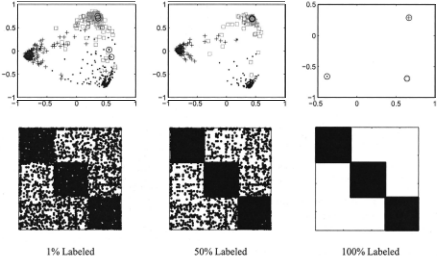
It was suggested in Section 4.2 that the Markov chain de scribed above will have cliques, that is, subsets of nodes in the graph that are internally fast-mixing, but are not mutu ally fast-mixing. Figure 4 shows the thresholded sparsity pat tern for the affinity matrices for the 3 Newgroups data set, as labeled data is added. The left matrix is the affinity matrix for 1% labeled data. Even the underlying similarities show block-like behavior, if weakly. To the extent that the unla beled data gives a block-like affinity matrix, clusters natu rally exist in the data; this is the basis for spectral clustering. The subsequent matrices have increasing fractions of data la beled. The effect of adding labeled data is to sharpen and coerce the natural clusters into the desired classes. As more labels are added, the blocks become clearer, the cliques be come stronger, and, in the limit of 100% labeled data, the interested reader will never accidently jump from a document of one topic to one of another.
0.6-
0.9
0.8 :
0.7"
0
- Spectral Classifier
1
~~~N~a~iv~eB~a~vee~s~C~Ias~si~fie~r~
0.2 0.4 0.6 0.8
(b) Adding Labeled Data
0.8 r------------------,
0.6~
0.4
0.2 . .------------~
0 L_~-- ~Na=iv=e=Ba~y=es=C=Ia~ss=:ifie=r~
0
: ~- Spectral Classifier l
0.1
0.2
0.3
0.4
(b) Adding Labeled Data
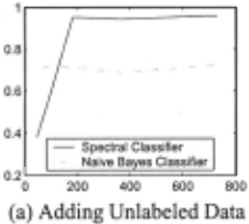
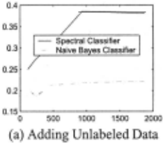
Figure 3: Categorization accuracy on the 20 NEWSGROUPS task as the (a) amount of unlabeled data and (b) traction of labeled data increases.
Accuracies
To validate the utility of spectral classification, we performed the following experiments on the 20 NEWSGROUPS data set.
We built two batch classifiers. The first was a standard multinomial Naive Bayes (NB) classifier with standard add one smoothing. The second was a spectral classifier as de scribed above, which used a single-nearest neighbor classifier to perform the final classification in the spectral space. The affinity matrix A was the thresholded cosine similarity be tween documents. 5 We note here that the thresholding is im portant, since it weakens the effect of outliers. Furthermore, it saves space and computation time, since the resulting affinity matrix is sparse.
We split the data into a labeled training set and an unla beled test set. For classification, the spectral classifier pro cessed both the training and test set, but was evaluated on the test set only.
Figure 2(a) shows the effect of using a sample of 12 docu ments from the 3 NEWSGROUPS data as a labeled training set, with an increasing number of unlabeled documents as a test set. The accuracy of the NB classifier is, of course, constant up to sampling variation, since it discards unlabeled data. The spectral classifier is more accurate than the NB classifier when given sufficiently many additional unlabeled documents to incorporate.
5 For each document, we take the most similar 20 documents, and put those similarities in the appropriate row and column. All other entries are 0.
Figure 2(b) shows the effect of supplying increasingly large fractions of the 3 NEWSGROUPS data set as labeled training instances, and using the remainder of the data set as test instances. The spectral classifier outperforms Naive Bayes, more substantially so when there is little labeled data. Figures 3(a) and (b) show the same graphs for the 20 NEWS GROUPS data set. Again, spectral classification performs well, especially when less than 10% of the data is labeled. It should be noticed that, for this data set, Naive Bayes out performs the spectral classifier in the strongly supervised case (> 15% labeled data). The strength of Spectral Learning lies in incorporating unlabeled data, and, for the strongly super vised case, this is of less value.
Spectral Space
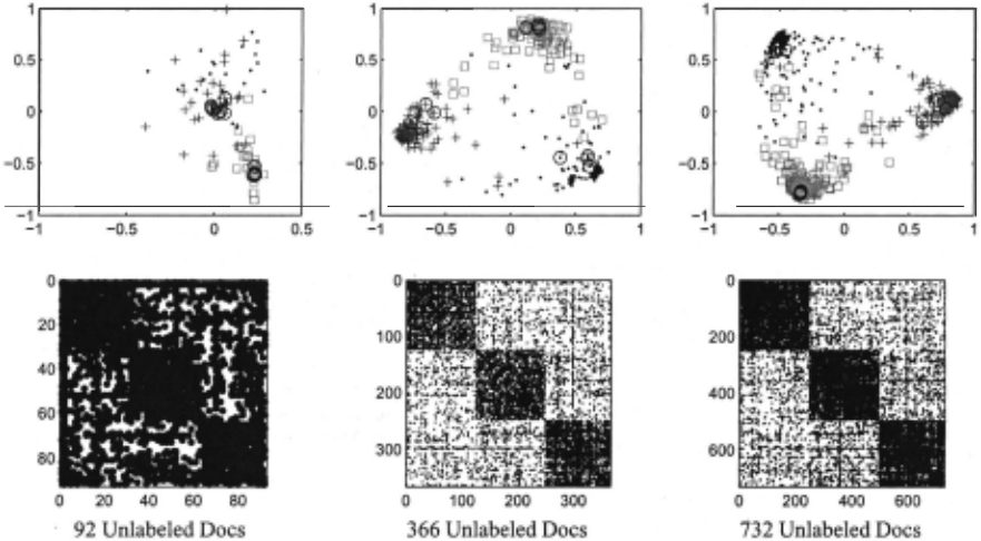
To further investigate the behavior of the spectral classi fier, we performed the following experiment. We took the 3 NEWSGROUPS data and labeled various fractions of each of the 3 classes. We then plotted each document's position in the resulting 3-dimensional spectral space (the space of the rows of the matrix X as defined by our spectral learn ing algorithm). Figure 4 shows dimensions 2 and 3 of these plots. With no labels, the data does not tightly cluster. As we add labels (circled points), two things happen. First, the labeled points move close to same-labeled points, away from different-labeled points, and generally towards the outside, since they are "hubs" of the Markov process. Second, they pull the unlabeled points out radially along with them. This is effective in that it seems to pull the classes apart, even though the classes were not naturally very strong clusters in the un labeled data.
4.4 Related Work
In [Yu and Shi, 2001], a spectral grouping method, which they call "Grouping with Bias", is presented that allows for top-level bias, as in labeled data. They formulate the problem as a constrained optimization problem, where the optimal par tition is sought, subject to the constraint that the normalized cut values of any two nodes that are preassigned to the same class should be the same.
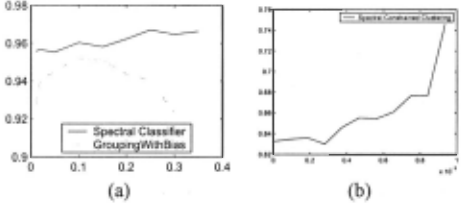
The main drawback with the algorithm in [Yu and Shi, 2001] is that it only constrains same-labeled data points. The algorithm we present here benefits from the zeros in the spar sity pattern introduced by differently-labeled pairs. Further more, it should be noted that, in the multi-class case, labeled sets combinatorialy tend to embody more differently-labeled pairs than same-labeled pairs. The other drawback to not us ing the information given by differently-labeled points is that the trivial partition (all points in one cluster) will satisfy the constraints, even when many points are labeled. In fact, when all the data is labeled, it is likely that the partition found by the Grouping with Bias algorithm will be the trivial partition. Figure 6(a) shows that our Spectral Classifier outperforms the Grouping with Bias algorithm for the 3 NEWSGROUPS data set. In fact, Grouping with Bias started performing slightly worse when a large fraction of the data was labeled.
5 Constrained Spectral Clustering
Recently, there has been interest in constrained clustering [Wagstaff and Cardie, 2000; Klein et a/., 2002], which in volves clustering with two types of pairwise constraints:
- Must-links: two items are known to be in the same class.
- Cannot-links: two items are in different classes.
Constrained clustering allows one to do exploratory data analysis when one has some prior knowledge, but not class la bels. The classifier presented in section 4 can be easily modified for this kind of prior knowledge: we have been reducing labeling information to pairwise information during affinity modification all along.
Specifically, the affinity matrix is now defined as follows:
- Define the affinity matrix A as before.
- For each pair of must-linked points (i, j) assign the val ues AiJ = AJ; = 1.
- For each pair of cannot-linked points (i , j) that are in different classes, assign the values AiJ = A Ji = 0.
- Normalize N = -d 1 (A+ dmaxl- D). max
This is equivalent to the imposing constraints step in [Klein eta/., 2002]. In this step, must-linked points are made more similar than any other pair of points in the data set, and cannot-linked points are made more dissimilar than any pair of points in the data set.
The spectral constrained clustering algorithm proceeds just as the other spectral clustering algorithms presented here; the only difference is that it uses the modified normalized affinity matrix presented in this section.
Figure 6(b) shows a plot of accuracy vs. number of con straints for the 3 NEWSGROUPS data set using spectral con strained clustering. The accuracy is measured by the con strained Rand index [Klein et a/., 2002; Wagstaff and Cardie, 2000]. The accuracy increases with number of constraints, showing that the spectral constrained clustering can effec tively use constraints to better cluster data.
6 Conclusion
We present here a probabilistic model and an associated spec tral learning algorithm that is able to work for the unsuper vised, semi-supervised, and fully-supervised learning prob lems. We show that this algorithm is able to cluster well, and further is able to effectively utilize prior knowledge, either given by pairwise constraints or by labeled examples.
Acknowledgments
This paper is based on research supported in part by the Na tional Science Foundation under Grant No. IIS-0085896, and by the Research Collaboration between NTT Communication Science Laboratories, Nippon Telegraph and Telephone Cor poration and CSLI, Stanford University (research project on Concept Bases for Lexical Acquisition and Intelligently Rea soning with Meaning).
@inproceedings{ijcai2003p83,
  title     = {Spectral Learning},
  author    = {Kamvar, Sepandar D. and Klein, Dan and Manning, Christopher D.},
  booktitle = {Proceedings of the Eighteenth International Joint Conference on
               Artificial Intelligence, {IJCAI-03}},
  publisher = {International Joint Conferences on Artificial Intelligence},
  editor    = {Georg Gottlob and Toby Walsh},
  pages     = {561--565},
  year      = {2003},
  url       = {https://ijcai.org/proceedings/2003/83},
}
TY - CPAPER TI - Spectral Learning AU - Kamvar, Sepandar D. AU - Klein, Dan AU - Manning, Christopher D. T2 - Proceedings of the Eighteenth International Joint Conference on Artificial Intelligence, IJCAI-03 PB - International Joint Conferences on Artificial Intelligence PY - 2003 SP - 561 EP - 565 UR - https://ijcai.org/proceedings/2003/83 ER -Copied
Machine-readable versions of this paper, for tools and AI agents:





