
Constructing Diverse Classifier Ensembles using Artificial Training Examples
Proceedings of the Eighteenth International Joint Conference on Artificial Intelligence. Pages 505-511.
© 2003 International Joint Conferences on Artificial Intelligence
Abstract
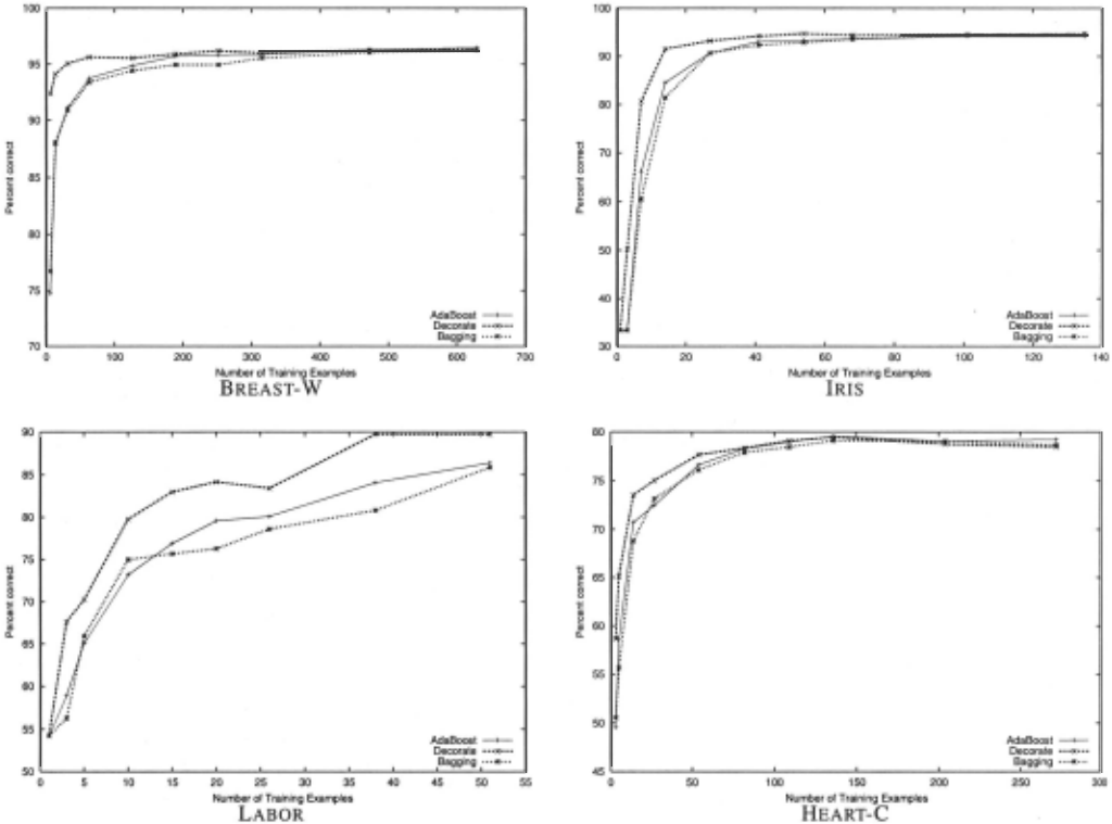
Ensemble methods like bagging and boosting that combine the decisions of multiple hypotheses are some of the strongest existing machine learning methods. The diversity of the members of an ensemble is known to be an important factor in determining its generalization error. This paper presents a new method for generating ensembles that directly constructs diverse hypotheses using additional artificially-constructed training examples. The technique is a simple, general metalearner that can use any strong learner as a base classifier to build diverse committees. Experimental results using decision-tree induction as a base learner demonstrate that this approach consistently achieves higher predictive accuracy than both the base classifier and bagging (whereas boosting can occasionally decrease accuracy), and also obtains higher accuracy than boosting early in the learning curve when training data is limited.
- [Bauer and Kohavi, 1999] E. Bauer and R. Kohavi. An empirical comparison of voting classification algorithms: Bagging, boosting and variants. Machine Learning, 36, 1999.
- [Blake and Merz, 1998] C. L. Blake and C. J. Merz. UCI repository of machine learning databases. http://www.ics.uci.edurmlearn/MLRepository.html, 1998. Link
- [Breiman, 1996] Leo Brei man. Bagging predictors. Machine Learning, 24(2):123-140, 1996.
- [Cohn et al., 1994] D. Cohn, L. Atlas, and R. Ladner. Im- proving generalization with active learning. Machine Learning, 15(2):201-221, 1994.
- [Cunningham and Carney, 2000] P. Cunningham and J. Car- ney. Diversity versus quality in classification ensembles based on feature selection. In lith European Conference on Machine Learning, pages 109-116, 2000.
- [Dietterich, 2000] T. Dietterich. Ensemble methods in ma- chine learning. In J. Kittler and F. Roli, editors, First Inter- national Workshop on Multiple Classifier Systems, Lecture Notes in Computer Science, pages 1-15. Springer-Verlag, 2000.
- [Freund and Schapire, 1996] Yoav Freund and Robert E. Schapire. Experiments with a new boosting algorithm. In Proceedings of the 13th International Conference on Ma- chine Learning, July 1996.
- [Hastie et al., 2001] Trevor Hastie, Robert Tibshirani, and Jerome Friedman. The Elements of Statistical Learning. Springer Verlag, New York, August 2001.
- [Krogh and Vedelsby, 1995] A. Krogh and J. Vedelsby. Neu- ral network ensembles, cross validation and active learn- ing. In Advances in Neural Information Processing Sys- tems 7, 1995.
- [Kuncheva and Whitaker, 2002] L. Kuncheva and C. Whitaker. Measures of diversity in classifier ensem- bles and their relationship with the ensemble accuracy. submitted, 2002.
- [Liu and Yao, 1999] Y. Liu and X. Yao. Ensemble learning via negative correlation. Neural Networks, 12, 1999.
- [Nigam et al., 2000] K. Nigam, A. K. McCallum, S. Thrun, and T. Mitchell. Text classification from labeled and unla- beled documents using EM. Machine Learning, 39:103- 134,2000.
- [Opitz and Maclin, 1999] David Opitz and Richard Maclin. Popular ensemble methods: An empirical study. Journal of Artificiallntelligence Research, 11:169-198, 1999.
- [Opitz and Shavlik, 1996] D. Opitz and J. Shavlik. Actively searching for an effective neural-network ensemble. Con- nection Science, 8, 1996.
- [Quinlan, 1993] J. Ross Quinlan. C4.5: Programs forMa- chine Learning. Morgan Kaufmann, San Mateo,CA, 1993.
- [Quinlan, 1996] J. Ross Quinlan. Bagging, boosting, and C4.5. In Proceedings of the 13th National Conference on Artificial Intelligence, August 1996.
- [Rosen, 1996] B. Rosen. Ensemble learning using decorre- lated neural networks. Connection Science, 8, 1996.
- [Webb, 2000] G. Webb. Multiboosting: A technique for combining boosting and wagging. Machine Learning, 40, 2000.
- [Witten and Frank, 1999] Ian H. Witten and Eibe Frank. Data Mining: Practical Machine Learning Tools and Techniques with Java Implementations. Morgan Kauf- mann, San Francisco, 1999.
- [Zenobi and Cunningham, 2001] G. Zenobi and P. Cunning- ham. Using diversity in preparing ensembles of classifiers based on different feature subsets to minimize generaliza- tion error. In Proceedings of the European Conference on Machine Learning, 2001.
References were extracted automatically from the PDF and may contain errors.
Full text extracted automatically from the PDF; figures, tables and equations may differ. The PDF is the version of record.
1 Introduction
One of the major advances in inductive learning in the past decade was the development of ensemble or committee ap proaches that learn and retain multiple hypotheses and com bine their decisions during classification [Dietterich, 2000]. For example, boosting [Freund and Schapire, 1996], an en semble method that learns a series of "weak" classifiers each one focusing on correcting the errors made by the previous one, has been found to be one of the currently best generic inductive classification methods [Hastie et al., 2001].
Constructing a diverse committee in which each hypothesis is as different as possible (decorrelated with other members of the ensemble) while still maintaining consistency with the training data is known to be a theoretically important property of a good committee [Krogh and Vedelsby, 1995]. Although all successful ensemble methods encourage diversity to some extent, few have focused directly on the goal of maximizing diversity. Existing methods that focus on achieving diversity [Opitz and Shavlik, 1996; Rosen, 1996] are fairly complex and are not general meta-learners like bagging [Breiman, 1996] and boosting that can be applied to any base learner to produce an effective committee [Witten and Frank, 1999].
We present a new meta-learner (DECORATE, Diverse En semble Creation by Oppositional Relabeling of Artificial Training Examples) that uses an existing "strong" learner (one that provides high accuracy on the training data) to build an effective diverse committee in a fairly simple, straightfor ward manner. This is accomplished by adding different ran domly constructed examples to the training set when building new committee members. These artificially constructed ex amples are given category labels that disagree with the cur rent decision of the committee, thereby easily and directly increasing diversity when a new classifier is trained on the augmented data and added to the committee.
Boosting and bagging provide diversity by sub-sampling or re-weighting the existing training examples. If the train ing set is small, this limits the amount of ensemble diversity that these methods can obtain. DECORATE ensures diversity on an arbitrarily large set of additional artificial examples. Therefore, one hypothesis is that it will result in higher gen eralization accuracy when the training set is small. This pa per presents experimental results on a wide range of UCI data sets comparing boosting, bagging, and DECORATE, all using 148 decision-tree induction (a Java implementation of C4.5 [Quinlan, 1993] introduced in [Witten and Frank, 1999]) as a base learner. Cross-validated learning curves support the hy pothesis that "DECORATEd trees" generally result in greater classification accuracy for small training sets.
2 Ensembles and Diversity
In an ensemble, the combination of the output of several classifiers is only useful if they disagree on some inputs [Krogh and Vedelsby, 1995]. We refer to the measure of disagreement as the diversity of the ensemble. There have been several methods proposed to measure ensemble diver sity [Kuncheva and Whitaker, 2002] - usually dependent on the measure of accuracy. For regression, where the mean squared error is commonly used to measure accuracy, vari ance can be used as a measure of diversity. So the diver sity of the ith classifier on example x can be defined as di(x) = [Ci(x) - C*(x)J2, where Ci(x) and C*(x) are the predictions of the ith classifier and the ensemble respec tively. For this setting Krogh et al [1995] show that the gen eralization error, E, of the ensemble can be expressed as E = E-D, where E and Dare the mean error and diversity of the ensemble respectively.
For classification problems, where the 011 loss function is most commonly used to measure accuracy, the diversity of the ith classifier can be defined as:
However, in this case the above simple linear relationship does not hold between E, E and b. But there is still strong reason to believe that increasing diversity should decrease en semble error [Zenobi and Cunningham, 2001]. The underly ing principle of our approach is to build ensembles of classi fiers that are consistent with the training data and maximize diversity as defined in ( 1 ).
3 DECORATE: Algorithm Definition
In DECORATE (see Algorithm 1), an ensemble is generated iteratively, learning a classifier at each iteration and adding it to the current ensemble. We initialize the ensemble to contain the classifier trained on the given training data. The classifiers in each successive iteration are trained on the original training data and also on some artificial data. In each iteration artifi cial training examples are generated from the data distribu tion; where the number of examples to be generated is spec ified as a fraction, Rsize, of the training set size. The labels for these artificially generated training examples are chosen so as to differ maximally from the current ensemble's predic tions. The construction of the artificial data is explained in greater detail in the following section. We refer to the labeled artificially generated training set as the diversity data. We train a new classifier on the union of the original training data and the diversity data. If adding this new classifier to the cur rent ensemble increases the ensemble training error, then we reject this classifier, else we add it to the current ensemble. This process is repeated until we reach the desired committee size or exceed the maximum number of iterations.
To classify an unlabeled example, x, we employ the fol lowing method. Each base classifier, C;, in the ensemble C* provides probabilities for the class membership of x. If Pc, ,y(x) is the probability of example x belonging to class y according to the classifier C;, then we compute the class membership probabilities for the entire ensemble as:
where Py(x) is the probability of x belonging to class y. We then select the most probable class as the label for x i.e. C*(x) = argmaxyEY Py(x)
3.1 Construction of Artificial Data
We generate artificial training data by randomly picking data points from an approximation of the training-data distribu tion. For a numeric attribute, we compute the mean and stan dard deviation from the training set and generate values from the Gaussian distribution defined by these. For a nominal attribute, we compute the probability of occurrence of each distinct value in its domain and generate values based on this distribution. We use Laplace smoothing so that nominal at tribute values not represented in the training set still have a non-zero probability of occurrence. In constructing artificial data points, we make the simplifying assumption that the at tributes are independent. It is possible to more accurately es timate the joint probability distribution of the attributes; but this would be time consuming and require a lot of data.
In each iteration, the artificially generated examples are la beled based on the current ensemble. Given an example, we first find the class membership probabilities predicted by the ensemble, replacing zero probabilities with a small non-zero value. Labels are then selected, such that the probability of selection is inversely proportional to the current ensemble's predictions.
Algorithm 1 The DECORATE algorithm
Input:
BaseLearn- base learning algorithm
T - set of m training examples < ( x1 , yl), ... , ( Xm, Ym) > with labels Yi E Y .
Csize -desired ensemble size
I max -maximum number of iterations to build an ensemble Rsize -factor that determines number of artificial examples to generate
- i = 1
- trials= 1
- Ci = BaseLearn(T)
- Initialize ensemble, C* = { C;}
- 2:. ·ET<C*( · ·);o!y · l 5. Compute ensemble error, E = 2 m 2 2
- While i < Csize and trials < Imax
- Generate R size x ITI training examples, R, based on distribution of training data
- Label examples in R with probability of class labels inversely proportional to C* 's predictions
- T = TUR
- C' = BaseLearn(T)
- C* = C* U{C'}
- T = T - R, remove the artificial data
- Compute training error, ~:', of C* as in step 5
- IfE 1 ~ E
- i = i + 1
- E = E 1
- otherwise,
- C* = C*- {C'}
- trials = trials + 1
4 Experimental Evaluation
4.1 Methodology
To evaluate the performance of DECORATE we ran experi ments on 15 representative data sets from the UCI repository [Blake and Merz, 1998] used in similar studies [Webb, 2000;
Quinlan, 1996]. We compared the performance of DECO RATE to that of Adaboost, Bagging and J48, using J48 as the base Ieamer for the ensemble methods and using the Weka implementations of these methods [Witten and Frank, 1999]. For the ensemble methods, we set the ensemble size to 15. Note that in the case of DECORATE, we only specify a max imum ensemble size, the algorithm terminates if the number of iterations exceeds the maximum limit even if the desired ensemble size is not reached. For our experiments, we set the maximum number of iterations in DECORATE to 50. We ran experiments varying the amount of artificially generated data, Rsize; and found that the results do not vary much for the range 0.5 to 1. However, Rsize values lower than 0.5 do adversely affect DECORATE, because there is insufficient ar tificial data to give rise to high diversity. The results we report are for Rsize set to 1, i.e. the number of artificially generated examples is equal to the training set size.
The performance of each learning algorithm was evaluated using 10 complete 10-fold cross-validations. In each 10-fold cross-validation each data set is randomly split into 10 equal size segments and results are averaged over 10 trials. For each trial, one segment is set aside for testing, while the remaining data is available for training. To test performance on vary ing amounts of training data, learning curves were generated by testing the system after training on increasing subsets of the overall training data. Since we would like to summarize results over several data sets of different sizes, we select dif ferent percentages of the total training-set size as the points on the learning curve.
To compare two learning algorithms across all domains we employ the statistics used in [Webb, 2000], namely the win/draw/loss record and the geometric mean error ratio. The win/draw/loss record presents three values, the number of data sets for which algorithm A obtained better, equal, or worse performance than algorithm B with respect to classi fication accuracy. We also report the statistically significant win/draw/loss record; where a win or loss is only counted if the difference in values is determined to be significant at the 0.05 level by a paired t-test. The geometric mean error ratio
is defined as vrr7=1 ~, where EA and EB are the mean errors of algorithm A and B on the same domain. If the ge ometric mean error ratio is less than one it implies that algo rithm A performs better than B, and vice versa. We compute error ratios so as to capture the degree to which algorithms out-perform each other in win or loss outcomes.
4.2 Results
Our results are summarized in Tables 1-3. Each cell in the tables presents the accuracy of DECORATE versus another al gorithm. If the difference is statistically significant, then the larger of the two is shown in bold. We varied the training set sizes from 1-100% of the total available data, with more points lower on the learning curve since this is where we expect to see the most difference between algorithms. The bottom of the tables provide summary statistics, as discussed above, for each of the points on the learning curve.
DECORATE has more significant wins to losses over Bag ging for all points along the learning curve (see Table 2).
DECORATE also outperforms Bagging on the geometric mean ratio. This suggests that even in cases where Bagging beats DECORATE the improvement is less than DECORATE's im provement on Bagging on the rest of the cases.
DECORATE outperforms AdaBoost early on the learning curve both on significant wins/draw/loss record and geomet ric mean ratio; however, the trend is reversed when given 75% or more of the data. Note that even with large amounts of training data, DECORATE's performance is quite competitive with Ada boost- given 100% of the data DECORATE produces higher accuracies on 6 out of 15 data sets.
It has been observed in previous studies [Webb, 2000; Bauer and Kohavi, 1999] that while AdaBoost usually sig nificantly reduces the error of the base learner, it occasionally increases it, often to a large extent. DECORATE does not have this problem as is clear from Table 1.
On many data sets, DECORATE achieves the same or higher accuracy as Bagging and AdaBoost with many fewer training examples. Figure 1 show learning curves that clearly demon strate this point. Hence, in domains where little data is avail able or acquiring labels is expensive, DECORATE has an ad vantage over other ensemble methods.
We performed additional experiments to analyze the role that diversity plays in error reduction. We ran DECORATE at 10 different settings of Rsize ranging from 0.1 to 1.0, thus varying the diversity of ensembles produced. We then com pared the diversity of ensembles with the reduction in gener alization error. Diversity of an ensemble is computed as the mean diversity of the ensemble members (as given by Eq. 1). We compared ensemble diversity with the ensemble error re duction, i.e. the difference between the average error of the ensemble members and the error of the entire ensemble (as in [Cunningham and Carney, 2000]). We found that the correla tion coefficient between diversity and ensemble error reduc tion is 0.6225 (p 1 « 10- 50 ), which is fairly strong. Further more, we compared diversity with the base error reduction, i.e. the difference between the error of the base classifier and the ensemble error. The base error reduction gives a better in dication of the improvement in performance of an ensemble over the base classifier. The correlation of diversity versus the base error reduction is 0.1552 (p « 10- 50 ) . We note that even though this correlation is weak, it is still a statistically significant positive correlation. These results reinforce our belief that increasing ensemble diversity is a good approach to reducing generalization error.
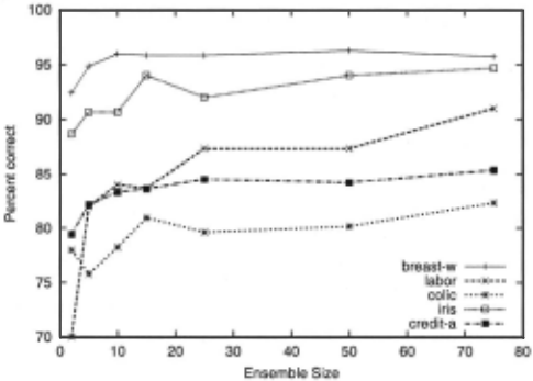
To determine how the performance of DECORATE changes with ensemble size, we ran experiments with increasing sizes. We compared results for training on 20% of available data, since the advantage of DECORATE is most noticeable low on the learning curve. Due to lack of space, we do not include the results for all 15 datasets, but present five representative datasets (see Figure 2). The performance on other datasets is similar. We note, in general, that the accuracy of DECORATE increases with ensemble size; though on most datasets, the performance levels out with an ensemble size of 10 to 25.
1 The p-value is the probability of getting a correlation as large as the observed value by random chance, when the true correlation is zero.
5 Related Work
There have been some other attempts at building ensembles that focus on the issue of diversity. Liu et al [ 1999] and Rosen [1996] simultaneously train neural networks in an ensemble using a correlation penalty term in their error functions. Opitz and Shavlik [1996] use a genetic algorithm to search for a good ensemble of networks. To guide the search they use an objective function that incorporates both an accuracy and diversity term. Zenobi et al [2001] build ensembles based on different feature subsets; where feature selection is done using a hill-climbing strategy based on classifier error and diversity. A classifier is rejected if the improvement of one of the metrics lead to a "substantial" deterioration of the other; where "substantial" is defined by a pre-set threshold.
In all these approaches, ensembles are built attempting to simultaneously optimize the accuracy and diversity of indi vidual ensemble members. However, in DECORATE, our goal is to minimize ensemble error by increasing diversity. At no point does the training accuracy of the ensemble go below that of the base classifier; however, this is a possibility with previous methods. Furthermore, none of the previous stud ies compared their methods with the standard ensemble ap proaches such as Boosting and Bagging ([Opitz and Shavlik, 1996] compares with Bagging, but not Boosting).
| Dataset | 1% | 2% | 5% | 10% | 20% | 30% | 40% | 50% | 75% | 100% |
|---|---|---|---|---|---|---|---|---|---|---|
| anneal audio autos breast-w credit-a Glass heart-c hepatitis colic iris labor lymph segment soybean splice | 75.29172.49 16.66/16.66 24.33/24.33 92.38174.73 71.78/69.54 31.69/31.69 58.66/49.57 52.33/52.33 59.85/52.85 33.33/33.33 54.27/54.27 48.39/48.39 67.94/52.43 19.37113.69 63.48/59.92 15/0/0 | 78.14175.31 23.73/23.07 29.6/29.01 94.12/87.34 74.83n7.46 35.86/32.96 65.11158.03 71.95/65.93 68.19/65.31 50.87/33.33 54.27/54.27 53.49/46.64 80.75n3.26 32.12/22.32 67.56/68.69 13/0/2 10/3/2 | 85.24/82.08 41.72/41.17 36.73/34.37 95.06/89.42 80.61/81.57 44.5/38.34 73.55/67.71 76.59172.75 74.91174.37 80.67/59.33 67.7/58.93 65.73/60.39 89.52/85.4 I 55.55/42.94 77.34177.49 13/0/2 11/4/0 | 92.26/89.28 55.42/51.67 42.89/41.22 95.64/92.21 83.09/82.35 55.4/46.62 75.05170.15 78.85178.25 78.45179.94 91.27/84.33 71.47/64.77 72.79/68.2 I 92.87/89.34 73.51159.04 82.62/82.58 14/0/1 | 96.48/95.57 64.09/60.59 52.2/50.53 95.55/93.09 84.38/84.29 61.77/54.16 77.66n3.44 80.28178.61 81.81/82.71 93.07/91.33 78.6170.07 74.57170.79 94.99/92.22 84.63174.49 88.2/87.98 14/0/1 | 97.36/96.47 67.62/64.84 59.86/53.92 95.91193.36 84.68/84.59 66.01160.63 78.34174.61 81.14178.63 82.47/83.41 94.4/92.73 81.67n3.7 78.84n3.58 95.82/93.37 88.52/81.59 90.46190.44 14/0/1 12/3/0 | 97.73/97.3 70.46/68.11 64.77/59.68 96.2/93.85 85.22/84.41 68.07/61.38 79.09174.78 81.53179.35 82.74/83.55 95.07/93 85.67175. I 7 78.37174.53 96.54/94.34 90.37/84.78 91.82/91.77 14/0/1 13/2/0 | 98.16/97.93 72.82170.77 68.6/65.24 96.01194.24 85.57/84.78 68.85/63.69 79.46175.62 81.68179.57 83.5/84.66 94.07/93.33 84.2175.8 78.31173.34 96.93/94.77 91.35/86.89 92.5/92.4 14/0/1 12/2/1 | 98.39/98.35 77.8175.15 78n3.15 96.28/94.65 85.61/85.43 72.73/67.53 78.74176.7 82.37179.04 83.93/85.18 94.67/94.07 87.53n7.4 78.06175.63 97.56/95.94 92.85/89.44 93.41/93.47 13/0/2 10/4/1 | 98.71/98.55 82.1n7.22 83.64/81.72 96.31195.01 85.93/85.57 72.77/67.77 78.48177.17 82.43179.22 85.24/85.16 94.93/94.73 89.5178.8 78.74176.06 98.02/96.79 93.81191.76 93.92/94.03 14/011 10/4/1 |
| Win/Draw/Loss Sig. W/D/L GM error ratio | 7/8/0 0.858 | 0.8649 | 0.8116 | 10/5/0 0.8098 | I 1/4/0 0.8269 | 0.8103 | 0.7983 | 0.8305 | 0.8317 | 0.8293 |
| Dataset | 1% | 2% | 5% | 10% | 20% | 30% | 40% | 50% | 75% | 100% |
|---|---|---|---|---|---|---|---|---|---|---|
| anneal audio autos breast-w credit-a Glass heart-c hepatitis colic iris labor lymph segment soybean splice | 75.29174.57 16.66/12.98 24.33/22.16 92.38176.74 71.78/69.54 31.69/24.85 58.66/50.56 52.33/52.33 58.37/53.14 33.33/33.33 54.27/54.27 48.39/48.39 67.03/55.88 19.51114.56 62.77/62.52 | 78.14176.42 23.73/23.68 29.6/28 94.12/88.07 74.83177.99 35.86/31.47 65.11155.67 72.14/63.18 66.58/63.83 50.27/33.33 54.27/54.27 53.62/47.11 81.16176.36 32.4/24.58 67.8172.36 13/0/2 | 85.24/82.88 41.72/38.55 36.73/35.88 95.06/90.88 80.61/82.58 44.5/40.87 73.55/68.77 76.8175.2 75.85176.44 80.67/60.47 67.63/56.27 65.06/60. I 2 89.61/87.42 55.36/47.46 77.37/80.5 12/0/3 | 92.26/89.87 55.42/51.34 42.89/44.65 95.64/93.4 83.09/83.9 55.4/49.6 91.53/81.4 I 110/4 | 96.48/95.67 64.09/61.76 52.2/54.32 93.2/90.67 11/0/4 | 97.36/96.89 67.62/66.9 59.86/59.67 83175.67 12/0/3 | 97.73/97.34 70.46170.29 64.77/65.6 96.2/94.95 68.07/66.3 78. I 91.84/92.4 11/0/4 | 98.16/97.78 72.82n3.07 68.6/69.88 96.01195.55 85.57/85.64 68.85/68.44 79.46179.1 I 83.19/81.06 83.1/84.47 94.4/93.6 83.43178.6 78.99176.98 96.93/95.82 91.4/89.22 92.41193.07 10/0/5 8/5/2 | 98.39/98.53 77.8n7.32 78n7.97 96.28/96.07 85.61/86.12 72.73172 78.74179.05 82.99/80.87 84.02/85.4 94.53/94.47 89.73/80.83 79.14176.8 97.58/96.78 92.75/91.56 93.44/94.06 10/0/5 | 98.71/98.83 82.1180.71 83.64/83.12 96.31/96.3 85.93/85.96 72.77174.67 78.48178.68 82.62/81.34 84.69/85.34 94.67/94.73 89.73/85.87 79.08177.97 98.03/97.41 93.89/92.7 I 93.92/94.53 8/017 |
| Win/Draw/Loss | 91511 | |||||||||
| 15/0/0 | ||||||||||
| I | 95.55/94.42 | 95.91194.95 | ||||||||
| 84.38/85.13 | 84.68/85.78 | 85.22/85.59 | ||||||||
| 61.77/58.9 | 66.01164.35 | |||||||||
| 75.05173.17 | 77.66176.12 | 78.34177.9 | 79.09178.44 | |||||||
| 79.48178.64 | 80.7/80.42 | 81.81/81.07 | 81.65/81.22 | |||||||
| 79.54/80.06 | 81.33/83.04 | 82.47/83.58 | 83.02/83.98 | |||||||
| 94.2/92.33 | 94.73/92.87 | |||||||||
| 70.23/65.9 | 79.77174.97 | 84.17176.27 | ||||||||
| 71.2/69.68 | 76.74n3.6 | 78.84176.58 | 7177.68 | |||||||
| 92.83/91.01 | 94.88/93.4 | 95.94/94.65 | 96.47/95.26 | |||||||
| 73.06/65.45 | 85.14179.29 | 88.27/85.05 | 90.22/87.89 | |||||||
| 82.55/85.44 | 88.24/89.5 | 90.47/91.44 | ||||||||
| Sig. W/D/L | 817/0 | 10/3/2 | 10/3/2 | 10/2/3 | 8/4/3 | 617/2 | 517/3 | 4/9/2 | ||
| GM error ratio | 0.8727 | 0.8785 | 0.8552 | 0.8655 | 0.8995 | 0.9036 | 0.8979 | 0.9214 | 0.9312 | 0.9570 |
Compared to boosting, which requires a "weak" base learner that does not completely fit the training data (boosting terminates once it constructs a hypothesis with zero training error), DECORATE requires a strong learner, otherwise the ar tificial diversity training data may prevent it from adequately fitting the real data. When applying boosting to strong base learners, they must first be appropriately weakened in order to benefit from boosting. Therefore, DECORATE may be a preferable ensemble meta-learner for strong learners.
To our knowledge, the only other ensemble approach to uti lize artificial training data is the active learning method intro duced in [Cohn et al., 1994]. The goal of the committee here is to select good new training examples rather than to improve accuracy using the existing training data. Also, the labels of the artificial examples are selected to produce hypotheses that more faithfully represent the entire version space rather than to produce diversity. Cohn's approach labels artificial data ei ther all positive or all negative to encourage, respectively, the learning of more general or more specific hypotheses.
6 Future Work and Conclusion
In our current approach, we are encouraging diversity using artificial training examples. However, in many domains, a large amount of unlabeled data is already available. We could exploit these unlabeled examples and label them as diversity data. This would allow DECORATE to act as a form of semi supervised learning that exploits both labeled and unlabeled data [Nigam et al., 2000].
Our current study has used J48 as a base learner; how ever, we would expect similarly good results with other base learners. Decision-tree induction has been the most com monly used base learner in other ensemble studies, but there has been some work using neural networks and naive Bayes [Bauer and Kohavi, 1999; Opitz and Maclin, 1999]. Exper iments on "DECORATing" other learners is another area for future work.
By manipulating artificial training examples, DECORATE is able to use a strong base learner to produce an effective, diverse ensemble. Experimental results demonstrate that the approach is particularly effective at producing highly accurate ensembles when training data is limited, outperforming both bagging and boosting low on the learning curve. The empir ical success of DECORATE raises the issue of developing a sound theoretical understanding of its effectiveness. In general, the idea of using artificial or unlabeled examples to aid the construction of effective ensembles seems to be a promis ing approach worthy of further study.
| Dataset | 1% | 2% | 5% | 10% | 20% | 30% | 40% | 50% | 75% | 100% |
|---|---|---|---|---|---|---|---|---|---|---|
| anneal audio autos breast-w credit-a Glass heart-c hepatitis colic iris labor lymph segment soybean splice | 75.29n3.02 16.66/16.66 24.33/24.33 92.38n4.73 71.78/68.8 31.69/31.69 58.66/49.57 52.33/52.33 58.37/52.85 33.33/33.33 54.27/54.27 48.39/48.39 67.03/60.22 19.51/14.26 62.77/65.11 | 78.14n7.12 23.73/23.41 29.6/29.71 94.12/87.84 74.83n5.3 35.86/32.93 65.11158.65 72.14/65.93 50.27/33.33 54.27/54.27 53.62/46.64 81.16n7.38 32.4/23.36 67.8n3.9 11/0/4 | 85.24/87.51 41.72/40.24 36.73/34.2 44.5/40.71 76.8n3.01 80.67/66.2 89.61/88.5 77.3 13/0/2 | 92.26/94.16 55.42/52.7 70.23/65.1 1210/3 | 96.48/97.13 64.09/64.15 52.2/56.13 93.2190.73 10/0/5 | 97.36/97.95 67.62/68.91 59.86/62.2 94.2/93 83n6.9 10/0/5 4/9/2 | 97.73/98.54 70.46n3.07 96.2/95.84 85.22/84. 13 68.07/66.93 79.09n8.96 81.65/81.27 83.02n9.51 94.73/93.33 84.17n9.57 78.17/80.35 96.47/96.9 91.84/90.8 10/0/5 51515 | 98.16/98.8 72.82n5.92 68.6n2.03 96.01/95.87 85.57/84.58 68.85/68.69 79.46n9.55 83.19/82.63 83.1/80.22 94.4/93.53 83.43/80.1 78.99n9.88 96.93/97.23 91.4/90.89 92.41/90.78 9/0/6 5/6/4 | 98.39/99.23 77.8/81.74 78/80.28 96.28/96.3 85.61/84.93 n.73n4.69 78.74n9.06 82.99/83.24 84.02/80.59 94.53/94.2 89.73/84.07 79.14/80.96 97.58/98 92.75/92.57 93.44/92.63 6/0/9 3/6/6 | 98.71/99.68 82.1/84.52 83.64/85.28 96.31/96.47 85.93/85.42 n.11n6.06 78.48n9.22 82.62/82.71 84.69/81.93 94.67/94.2 89.73/86.37 79.08/81.75 98.03/98.34 93.89/92.88 93.92193.59 61019 |
| Win/Draw/Loss | 14/0/1 7nll | 11/212 | 10/3/2 | 7/6/2 | ||||||
| 42.89/43.28 | 64.77/69.14 | |||||||||
| 95.06/91.15 | 95.64/93.75 | 95.55/94.85 | 95.91/95.72 | |||||||
| 80.61n9.68 | 83.09/81.14 | 84.38/83.04 | 84.68/84.22 | |||||||
| 55.4/49.78 | 61.77/58.03 | 66.01/64.33 | ||||||||
| 73.ssno.71 | 75.osn2.5 | 77.66n6.65 | 78.34n8.26 | |||||||
| 79.48n6.95 | 80.7n9.44 | 81.8ln9.22 | ||||||||
| 66.58/67.18 | 75.85n2.85 | 79.s4n7.17 | 81.33n9.36 | 82.47n9.24 | ||||||
| 91.53/84.53 | ||||||||||
| 67.63/58.93 | 79.77n3.2 | |||||||||
| 65.06/60.54 | 71.2/69.57 | 76.74n4.16 | 78.84n8.62 | |||||||
| 92.83/92.71 | 94.88/95.01 | 95.94/96.03 | ||||||||
| 55.36/49.37 | 73.06/69.49 | 85.14/85.01 | 88.27/88.37 | 90.22/90.04 | ||||||
| 7/82.22 | 82.55/86.13 | 88.24/88.27 | 90.47/89.82 | |||||||
| Sig. W/D/L | 8/6/1 | 3/6/6 | ||||||||
| GM error ratio | 0.8812 | 0.8937 | 0.8829 | 0.9104 | 0.9407 | 0.9598 | 0.9908 | 0.9957 | 1.0377 | 1.0964 |
Acknowledgments
This work was supported by DARPA EELD Grant F3060201-2-0571.
@inproceedings{ijcai2003p75,
  title     = {Constructing Diverse Classifier Ensembles using Artificial Training Examples},
  author    = {Melville, Prem and Mooney, Raymond J.},
  booktitle = {Proceedings of the Eighteenth International Joint Conference on
               Artificial Intelligence, {IJCAI-03}},
  publisher = {International Joint Conferences on Artificial Intelligence},
  editor    = {Georg Gottlob and Toby Walsh},
  pages     = {505--511},
  year      = {2003},
  url       = {https://ijcai.org/proceedings/2003/75},
}
TY - CPAPER TI - Constructing Diverse Classifier Ensembles using Artificial Training Examples AU - Melville, Prem AU - Mooney, Raymond J. T2 - Proceedings of the Eighteenth International Joint Conference on Artificial Intelligence, IJCAI-03 PB - International Joint Conferences on Artificial Intelligence PY - 2003 SP - 505 EP - 511 UR - https://ijcai.org/proceedings/2003/75 ER -Copied
Machine-readable versions of this paper, for tools and AI agents:





