When Discriminative Learning of Bayesian Network Parameters Is Easy

1 Introduction

In recent years it has been recognized that for discriminative prediction tasks such as classification, we should use a 'su­ pervised' learning algorithm such as conditional likelihood maximization [Friedman et al., 1997; Ng and Jordan, 2001; Kontkanen et al., 2001; Greiner and Zhou, 2002]. Neverthe­ less, for Bayesian network models the parameters are cus­ tomarily determined using ordinary methods such as maxi­ mization of the joint (unsupervised) likelihood. One of the main reasons for this discrepancy is the difficulty in finding the global maximum of the conditional likelihood. In this pa­ per, we show· that this problem can be solved, as long as the underlying Bayesian network meets a particular additional condition, which is satisfied for many existing Bayesian­ network based models including Naive Bayes (NB), TAN (tree-augmented NB) and 'diagnostic' models [Kontkanen et al., 2001].

We consider domains of discrete-valued random variables. We find the maximum conditional likelihood parameters by logarithmic reparametrization. In this way, each conditional Bayesian network model is mapped to a logistic regression

° Centrum voor Wiskunde en Informatica (CWI) P.O. Box 94079 NL-1090 GB Amsterdam, The Netherlands. Peter.Grunwald@cwi.nl

model, for which the likelihood surface is known to be con­ cave. However, in some cases the parameters of this logis­ tic regression model are not allowed to vary freely. In other words, the Bayesian network model corresponds to a subset of a logistic regression model rather than the full model.

Our main result (Thm. 3 below) provides a general condi­ tion on the network structure under which, as we prove, the Bayesian network model is mapped to a full logistic regres­ sion model with freely varying parameters. Therefore, in the new parametrization the conditional log-likelihood becomes a concave function of the parameters that under our condi­ tion are allowed to vary freely over the convex set JRk. Now we can find the global maximum in the conditional likelihood surface by simple local optimization techniques such as hill climbing.

The result still leaves open the possibility that there are no network structures for which the conditional likelihood sur­ face has local, non-global maxima. This would make our con­ dition superfluous. Our second result (Thm. 4 below) shows that this is not the case: there are very simple network struc­ tures that do not satisfy our condition, and for which the con­ ditionallikelihood can exhibit local, non-global maxima.

Viewing Bayesian network (BN) models as subsets of lo­ gistic regression models is not new; it was done earlier in papers such as [Heckerman and Meek, 1997a; Ng and Jor­ dan, 2001; Greiner and Zhou, 2002]. Also, the concavity of the log-likelihood surface for logistic regression is known. Our main contribution is to supply the condition under which Bayesian network models correspond to logistic regression with completely freely varying parameters. Only then can we guarantee that there are no local maxima in the likelihood surface. As a direct consequence of our result, we show for the first time that the supervised likelihood of, for instance, the tree-augmented Naive Bayes (TAN) model has no local maxima.

This paper is organized as follows. In Section 2 we in­ troduce Bayesian networks and an alternative, so-called £­ parametrization. In Section 3 we show that this allows us to consider Bayesian network models as logistic regression models. Based on earlier results in logistic regression, we conclude that in the £-parametrization the supervised log­ likelihood is a concave function. In Section 4 we present our main results, giving conditions under which the two parametrizations correspond to exactly the same conditional distributions. Conclusions are summarized in Section 5; proofs of the main results are given in Appendix A.

2 Bayesian Networks and the £-model

We assume that the reader is familiar with the basics of the theory of Bayesian networks, see, e.g., [Pearl, 1988].

Consider a random vector X = (Xo, xl' ... ' XM' ), where each variable Xi takes values in {1, ... , ni}· Let B be a Bayesian network structure over X, that factorizes P(X) into

where p ai ~ {X 0 , . . . ' X M' } is the parent set of variable xi in B.

We are interested in predicting some class variable Xm for some m E {0, ... , M'} conditioned on all Xi, i =F m. Without loss of generality we may assume that m = 0 (i.e., X0 is the class variable) and that the children of Xo in B are {X 1, ... , X M} for some M :::; M'. For instance, in the so-called Naive Bayes model we have M = M' and the chil­ dren of the class variable X 0 are independent given the value of X0 . The Bayesian network model corresponding to B is the set of all distributions satisfying the conditional indepen­ dencies encoded in B. It is usually parametrized by vectors 8 8 with components of the form a~, lpa; defined by

where pai is any configuration (set of values) for the par­ ents Pai of Xi. Whenever we want to emphasize that each pai is determined by the complete data vector x = (xo, ... , XM· ), we write pai(x) to denote the configuration of Pai in B given by the vector x. For a given data vec­ tor x = (x0 , x1 , . . . , XM' ), we sometimes need to consider a modified vector where x0 is replaced by x~ and the other entries remain the same. We then write pai(x~, x) for the configuration of P ai given by ( x~, x1 , ... , x M').

We let M 8 be the set of conditional distributions P(Xo I xl' ... 'XM'' 8 8) corresponding to distributions P(Xo , ... 'XM' I 8 8 ) satisfying the conditional indepen­ dencies encoded in B. The conditional distributions in M 8 can be written as

extended to N outcomes by independence.

Given a complete data-matrix D = (x 1 , ... , xN), the con­ ditional log-likelihood, S 8 (D; 8 8 ), with parameters 8 8 is given by N

where

Note that in (3), and hence also in (4), all a~;ipa; with i > M (standing for nodes that are neither the class variable nor any of its children) cancel out, since for these terms we have pai(x) = pai(x~, x) for all x~. Thus the only relevant parameters for determining the conditional likelihood are of the form a~;lpa; with i E {0, . .. , M}, Xi E {1, ... , ni} and pai any configuration of parents Pai. We order these param­ eters lexicographically and define 8 8 to be the set of vectors constructed this way, with a~. lpa; > 0 and L::~:=l a~. lpa; = 1 for all i E {0, ... , M}, Xi and all values (configurations) of pai. Note that we require all parameters to be strictly positive.

The model M 8 does not contain any notion of the joint dis­ tribution: Terms such as P(Xi I Pai), where 0 < i :::; M', are undefined and neither are we interested in them. Our task is prediction of X0 given X 1 , ... , X M'. Heckerman and Meek call such models Bayesian regression/classification (BRC) models [Heckerman and Meek, 1997a; 1997b].

For an arbitrary conditional Bayesian network model M 8 , we now define the so-called £-model, another set of con­ ditional distributions P~Xo I xl' ... 'XM' ). This model, which we denote by M , is parametrized by vectors e£ in some set eL that closely resembles E> 8 . Each different M B gives rise to a corresponding M L, although we do not nec­ essarily have M B = M L. For each component e~. lpa; of each vector 8 8 E 8 8 , there is a corresponding component e~. lpa; of the vectors e£ E E)L. The components e~. lpa; take values in the range ( -oo, oo) rather than (0, 1). Each vector 8£ E E)L defines the following conditional distribution:

The model ML is the set of conditional distributions P(Xo I xl' ... 'XM'' e£) indexed bye£ E eL' extended toN outcomes by independence. Given a data-matrix D, let SL(D; eL) be the conditional log-likelihood with parameters e£' defined analogously to (4) with (6) in place of (3).

Proof From (3) and (6) we get that e£ defined by setting a~;ipa; = Jn a~, lpa; for all i, Xi and pai, indexes the same conditional distribution as e 8 . I

In words, all the conditional distributions that can be rep­ resented by parameters 8 8 E 8 8 can also be represented by farameters 8£ E E)L. The converse of Theorem 1, i.e., M ~ M 8 , is true only under some additional conditions on the network structure, as we explain in Section 4. First we take a closer look at the £-model.

3 The £-model Viewed as Logistic Regression

Although £-models are closely related to and in some cases formally identical to Bayesian network models, we can also think of them as predictors that combine the information of the attributes using the so-called softmax rule [Heckerman and Meek, 1997b; Ng and Jordan, 2001]. In statistics, such models have been extensively studied under the name of lo­ gistic regression models, see, e.g. [McLachlan, 1992, p.255] .

More precisely, let Xo = {1, ... , no} and let Y1, ... , Yk be real-valued random variables. The multiple logistic re­ gression model with dependent variable X 0 and covariates Y1, ... , Yk is defined as the set of conditional distributions

where the ,Bxol; are allowed to take on all values in !It This defines a conditional model parameterized in JRno ·k. Now, for i E {O, .. . ,M},xi E {1 , ... ,ni}andpaiinthesetofparent configurations of xi. let

The indicator random variables Y( x ;,pa;) thus obtained can be lexicographically ordered and renamed 1, . . . , k, which shows that each L-model corresponding to a Bayesian net­ work structure B as in (6) is formally identical to the logistic model (7) with dependent variable X0 and covariates given by (8). So, for all network structures B, the corresponding L­ model ML is the standard multiple logistic model, where the input variables for the logistic model are transformations of the input variables to the L-model, the transformation being determined by the network structure B.

It turns out that the conditional log-likelihood in the £­ parametrization is a concave function of the parameters:

Theorem 2. The parameter set eL is convex, and the con­ ditional log-likelihood SL(D; eL) is concave, though not strictly concave.

Proof The first part is obvious since each parameter can take values in ( -oo, oo ). Concavity of SL(D; eL) is a direct con­ sequence of the fact that multiple logistic regression models are exponential families; see, e.g., [McLachlan, 1992, p.260]. For an example showing that the conditional log-likelihood is not strictly concave, see [Wettig et al., 2002]. I

Remark. Non-strictness of the proven concavity may pose a technical problem in optimization. This can be avoided by assigning a strictly concave prior on the model parameters and then maximizing the 'conditional posterior' [Grunwald et al., 2002; Wettig et al., 2002] instead of the likelihood. One may also prune the model of weakly supported parame­ ters and/or add constraints to arrive at a strictly concave con­ ditional likelihood surface. Our experiments [Wettig et al., 2002] suggest that for small data samples this should be done in any case, in order to avoid over-fitting; see also Section 5. Any constraint added should of course leave the parameter space a convex set, e.g. a subspace of the full eL.

Corollary 1. There are no local, non-global, maxima in the likelihood surface of an L-model.

The conditions under which a global maximum exists are discussed in, e.g., [McLachlan, 1992] and references therein. A possible solution in cases where no maximum exists is to introduce a strictly concave prior as discusssed above.

The global conditional maximum likelihood parameters obtained from training data can be used for prediction of future data. In addition, as discussed in [Beckerman and Meek, 1997a], they can be used to perform model selec­ tion among several competing model structures using, e.g., the BIC or (approximate) MDL criteria. In [Beckerman and Meek, 1997a] it is stated that for general conditional Bayesian network models M 6 , "although it may be difficult to deter­ mine a global maximum, gradient-based methods[ ... ] can be used to locate local maxima". Theorem 2 shows that if the network structure B is such that the two models are equiva­ lent, M 6 = ML, we can find even the global maximum of the conditional likelihood by reparametrizing M 6 to the L­ model, and using some local optimization method. Thus, the question under which condition M 6 = ML becomes cru­ cial. It is this question we address in the next section.

Remark. Because the log-transformation is continuous, it follows (with some calculus) that, if M 6 = ML, then all maxima of the (concave) conditional likelihood in the £­ parameterization are global (and connected) maxima also in the original parametrization. Nevertheless, the likelihood sur­ face as a function of 8 6 E 0 6 has some unpleasant proper­ ties (see [Wettig et al., 2002]): it is not concave in general and, worse, it can have 'wrinkles': by these we mean con­ vex subsets eg of 0 6 , such that, under the constraint that 8 6 E eg, the likelihood surface does exhibit local, non­ global maxima. This suggests that it is com;utationally pre­ ferrable to optimize over eL rather than e 0 Empirical evi­ dence for this is reported in [Greiner and Zhou, 2002].

4 Main Result

By setting (}~; jpa; = In(}~; iva;, it follows that each distribu­ tion in M 6 is also in ML (Thm. 1). This suggests that, by doing the reverse transformation

we could also show that distributions in ML are also in M B 0 However, eL contains distributions that violate the 'sum-up-to-one constraint', i.e., for some eL E eL we have 2:::~;= 1 expB~;jpa; =f. 1 for some i E {0, ... , M'} and pai. Then the corresponding e 6 is not in 0 6 0 But, since the £­ parameterization is redundant (many different 8£ index the same conditional distribution P(· I ·) E ML), it may still be the case that the distribution P(· I ·, eL) indexed by eL is in M 6 . Indeed, it turns out that for some network struc­ tures B, the corresponding ML is such that each distribution in M L can be expressed by a parameter vector eL such that "'nx;_ 1 exp e£ 1 . = 1 for all i E {0, .. . , M'} and pai. In D ,- x , pa, that case, by (9), we do have M 6 = M L. Our main result is that this is the case if B satisfies the following condition:

Condition 1. For all j E {1, ... , M}, there exists Xi E Pai such that Pai ~ Pai U {Xi}.

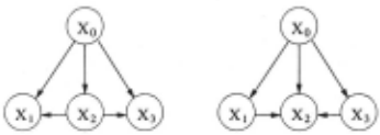
Remark. Condition 1 implies that the class X 0 must be a 'moral node', i.e., it cannot have a common child with a node it is not directly connected with. But Condition 1 demands more than that; see Figures 1 and 2.

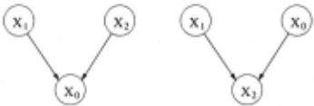
Example 1. Consider the Bayesian networks depicted in Fig­ ure 1. The leftmost network, B1 , satisfies Condition 1, the rightmost network, B2 , does not. Theorem 4 shows that the conditional likelihood surface of M 82 can have local max­ ima, implying that in this case M 8 =f. ML. 0

Examples of network structures that satisfy Condition 1 are the Naive Bayes (NB) and the tree-augmented Naive Bayes (TAN) models [Friedman et al., 1997]. The latter is a gen­ eralization of the former in which the children of the class variable are allowed to form tree-structures; see Figure 2.

Proposition 1. Condition 1 is satisfied by the Naive Bayes and the tree-augmented Naive Bayes structures.

Proof For Naive Bayes, we have Pai ~ {Xo} for all j E {1, ... , M} . For TAN models, all children of the class vari­ able have either one or two parents. For children with only one parent (the class variable) we can use the same argument as in the NB case. For any child Xi with two parents, let Xi be the parent that is not the class variable. Because Xi is also a child of the class variable, we have Pai ~ Pai U {Xi}. I

Condition 1 is also automatically satisfied if X 0 only has incoming arcs 1 ('diagnostic' models, see [Kontkanen et al., 2001 ]). For Bayesian network structures B for which the con­ dition does not hold, we can always add some arcs to arrive at a structure B' for which the condition does hold (for in­ stance, add an arc from xl to x3 in the rightmost network in Figure 2). Therefore, M 8 is always a subset of a larger model M B' for which the condition holds. We are now ready to present our main result (for proof see Appendix A):

Theorem 3. If B satisfies Condition 1, then M 8 = M L.

Together with Corollary 1, Theorem 3 shows that Condi­ tion 1 suffices to ensure that the conditional likelihood sur­ face of M 8 has no local (non-global) maxima. Proposition 1

1 It is easy to see that in that case the maximum conditional like­ lihood parameters may even be determined analytically.

now implies that, for example, the conditional likelihood sur­ face of TAN models has no local maxima. Therefore, a global maximum can be found by local optimization techniques.

But what about the case in which Condition 1 does not hold? Our second result, Theorem 4 (proven in Appendix A) says that in this case, there can be local maxima:

Theorem 4. Let B2 = X 1 -t X 2 +- X 0 be the network structure depicted in Figure 1 (right). There exist data sam­ ples such that the conditional likelihood has local, non-global maxima over M 82 .

The theorem implies that M L =f. M 82 . Thus, Condition 1 is not superfluous. We mat now ask whether our condition is necessary for having M = M 8 ; that is, whether ML =f. M 8 for all network structures that violate the condition. We plan to address this intriguing open question in future work.

5 Concluding Remarks

We showed that one can effectively find the parameters max­ imizing the conditional (supervised) likelihood of NB, TAN and many other Bayesian network models. We did this by showing that the network structure of these models satisfies our 'Condition 1 ', which ensures that the conditional distri­ butions corresponding to such models are equivalent to a par­ ticular multiple logistic regression model with unconstrained parameters. An arbitrary network structure can always be made to satisfy Condition 1 by adding arcs. Thus, we can embed any Bayesian network model in a larger model (with less independence assumptions) that satisfies Condition 1.

Test runs for the Naive Bayes case in [Wettig et al., 2002] have shown that maximizing the conditional likelihood in contrast to the usual practice of maximizing the joint (unsu­ pervised) likelihood is feasible and yields greatly improved classification. Similar results are reported in [Greiner and Zhou, 2002]. Our conclusions are also supported by theo­ retical analysis in [Ng and Jordan, 2001]. Only on very small data sets we sometimes see that joint likelihood optimization outperforms conditional likelihood, the reason apparently be­ ing that the conditional method is more inclined to over­ fitting. We conjecture that in such cases, rather than resorting to maximizing the joint instead of the conditional likelihood, it may be preferable to use a simpler model or simplify (i.e. prune or restrict) the model at hand and still choose its param­ eters in a discriminative fashion. In our setting, this would amount to model selection using the £-parametrization. This is a subject of our future research.