
Model-based Diagnosis of Hybrid Systems
Proceedings of the Eighteenth International Joint Conference on Artificial Intelligence. Pages 376-380.
© 2003 International Joint Conferences on Artificial Intelligence
Abstract
Recent years have seen a proliferation of embedded systems that combine a digital (discrete) supervisory controller with an analog (continuous) plant. Diagnosing faults in such hybrid systems , require techniques that are different from those used for discrete and continuous systems . In addition, these algorithms have to be deployed online to meet the real time requirements of embedded systems. This paper presents a methodology for online tracking and diagnosis of hybrid systems. We demonstrate the effectiveness of the approach with experiments conducted on the fuel transfer system of fighter aircraft.
- Alur, R., et al., Hybrid Automata-An Algorithmic Ap- proach to Specification and Verification of Hybrid Sys- tems, Lecture Notes in Computer Science: Hybrid Sys- tems I. 1994, Springer Verlag. p. 209-229. DIAGNOSIS
- Biswas, G. and X. Yu. A Formal Modeling Scheme for Continuous Systems: Focus on Diagnosis. in Proc. IJCAI 1993. Chambery, France, p 1474-1479. IJCAI
- Dearden, R. and D. Clancy. Particle Filters for Real- Time Fault Detection in Planetary Rovers. in Thirteenth Inti Wkshp . on Principles of Diagnosis, 2002.
- Semmer- ing, Austria.
- Gelb, A., Applied Optimal Estimation. 1979, Cam- bridge, MA, USA: MIT Press.
- Gertler, J.., Fault detection and Diagnosis in Engineer- ing Systems. 1998, New York: Marcel Dekker.
- Hofbaur, M.W. and B.C. Williams. Mode Estimation of Probabilistic Hybrid Systems. in Fifth International Workshop on Hybrid Systems: Computation and Control (HSCC '02). 2002. Stanford, CA, USA: Springer.
- Karnopp, D., D.L. Margolis, and R.C. Rosenberg, Sys- tem dynamics : modeling and simulation of mechatronic systems. 3rd ed. 2000, New York: Wiley.
- Koutsoukos, X., et al. Fault Modeling for Monitoring and Diagnosis of Sensor-Rich Hybrid Systems. in IEEE Conference on Decision and Control. 2001. Orlando, FL.
- Lunze, J. and J. Schroder, Sensor and Actuator Fault Diagnosis of Systems with Discrete Inputs and Outputs. in press, IEEE Transactions on Systems, Man, and Cy- bernetics, March, 2002.
- Manders, E. and G. Biswas. Transient Detection and Analysis for Diagnosis of Abrupt Faults in Continuous Dynamic Systems. in Inti Wkshp. on Intelligent Signal Processing (WISP 'OJ). 2001. Budapest, Hungary.
- Manders, E., P.J. Mosterman, and G. Biswas. Signal to Symbol Transformation techniques for Robust Diagno- sis in TRANSCEND. in Inti Wkshp on Principles of Diagnosis. 1999. Loch Awe, Scotland.
- Manders, E., et al. A combined Qualita- tive/Quantitative approach to efficient Fault Isolation in complex dynamic systems. in Inti. SafeProcess Sympo- sium, 2000. Budapest, Hungary, p.512-517.
- Mosterman, P.J. and G. Biswas, A Theory of discon- tinuities in Physical System Models. Journal of Franklin Institute, 1998. 335(B): p. 401-439.
- Mosterman, P.J. and G. Biswas, Diagnosis of Con- tinuous Valued Systems in Transient Operating Regions. IEEE Transactions on Systems, Man, and Cybernetics, 1999. 29: p. 554-565.
- Narasimhan, S., Model-based Diagnosis of Hybrid Systems, in Computer Science. 2002, Vanderbilt Univer- sity: Nashville.
- Narasimhan, S. and G. Biswas. An Approach to Model-Based Diagnosis of Hybrid Systems. in Hybrid Systems: Computation and Control (HSCC '02). 2002. Stanford, CA: Springer Verlag.
- Sampath, M., et al., Failure Diagnosis using Dis- crete-Event Models. IEEE Transactions on Control Sys- tems Technology, 1996. 4: p. 105-124.
References were extracted automatically from the PDF and may contain errors.
Full text extracted automatically from the PDF; figures, tables and equations may differ. The PDF is the version of record.
1 Introduction
This paper addresses the problem of designing and im plementing online monitoring and diagnosis systems for complex systems whose behavior is hybrid (discrete + continuous) in nature. Hybrid modeling covers naturally occurring systems, such as cell-cycle control systems in biology. They also capture the behavior of embedded systems that are common in the avionics, automotive, and robotics domains. This wide applicability of hybrid sys tems has inspired a great deal of research from both con trol theory and theoretical computer science.
We focus on a special class of embedded hybrid sys tems, characterized by continuous plant dynamics and a discrete supervisory controller. The plant dynamics are defined by continuous state variables associated with the components of the plant. The controller generates actua tor signals at discrete time points that can change the plant configuration by turning components ON and OFF, and changing component parameter values and the set points of regulators. Therefore, hybrid system models have to seamlessly integrate discrete and continuous be havior analyses using multiple system models. As a re sult, tasks like monitoring, fault diagnosis, and control require appropriate model selection and switching to be performed online as system behavior evolves.
This paper discusses methodologies for the model based diagnosis (MBD) of hybrid systems. Current tech niques in MBD apply well to dynamic systems whose behavior is modeled with discrete event [9, 17], or con-
Gautam Biswas
Dept. of EECS & ISIS Vanderbilt University Nashville, TN 3 723 5 gautam.biswas@vanderbilt.edu
tinuous models [5, 14]. Discrete event approaches to hy brid system diagnosis are based on abstractions of nomi nal and faulty behavior system behavior into event trajec tories. This process may result in loss of information critical for fault isolation and control. Our work in con tinuous diagnosis has demonstrated that behavior tran sients are the key to quick diagnosis of abrupt faults[ 1 0]. It may also be computationally expensive to pre enumerate all possible nominal and faulty behavior tra jectories. Traditional algorithms for continuous diagnosis use a single model that does not accommodate discrete changes. Therefore, discrete effects of mode changes have to be modeled by complex continuous non-linear functions that are hard to analyze online in real time.
Recent work on diagnosis of hybrid systems [3 , 6, 8] has focused on discrete faults, and requires the pre enumeration of the model in all modes to perform diag nosis. We present an online model-based diagnosis meth odology for parametric faults in hybrid systems that is based on tracking hybrid behaviors (continuous behaviors interspersed with discrete changes), but unlike hybrid automata models [1] pre-enumeration of all system modes is avoided by generating models at runtime as mode switches occur.
The fault isolation task has to take into account possi ble mode changes during diagnostic analysis. The occur rence of a fault necessarily implies that one no longer has a correct model of system behavior; therefore, mode changes cannot be correctly predicted. To address this, the fault isolation task incorporates a search process, where mode changes may have to be hypothesized and incorporated into the consistency-based diagnosis scheme. The fault isolation process becomes even more complicated if fault detection is delayed, and the diagno sis algorithm has to roll back modes to identify the mode in which the fault occurred. We have developed a generic tracking, fault detection, and fault isolation scheme, which address all of the issues we have outlined above. The rest of the paper presents our hybrid modeling, track ing, and diagnosis scheme for solving the hybrid diagno sis problem.
2 Unified Modeling Framework
We use a unified modeling framework called hybrid bond graphs that extends continuous bond graph modeling [7]
to provide compact representations for hybrid models. Its component based and hierarchical representation is ex pressed as topological structures that facilitate causal analysis of system dynamics. It also provides standard techniques for deriving state space and input output equa tion formulations that are suitable for tracking and esti mation tasks [ 15].
2.1 Bond Graphs
A bond graph (BG) is a domain-independent topological representation that captures energy-based interactions among the different physical processes that make up the system. The vertices in the graph represent subsystems modeled as generic physical processes: capacities, iner tias, and dissipators that can have linear and non-linear behaviors. Bonds are energy pathways by which subsys tems/processes exchange energy in the system. Two addi tional types of vertices (0 and 1 junctions) represent do main independent generalizations of Kirchoffs laws and are used as connection points between the sub-systems. There exist systematic techniques to construct the bond graph from the system description [2].
2.2 Hybrid Bond Graphs
Additional mechanisms are introduced into the continu ous BG language to include discrete transitions and model switching. We use switched junctions proposed by Mosterman and Biswas [13], where each junction in the bond graph may be switched on (activated) and off (de activated) . An activated junction behaves like a conven tional BG junction. All the bonds incident on a junction turned off are made inactive, and hence do not play any part in the system dynamics. Note that activating or de activating junctions affect the behavior of adjoining junc tions.
A Finite State Automaton (FSA) implements the junc tion switching function. The FSA may have several states, and each state maps to either the off mode (i.e., it causes the junction to turn off) or the on mode (i.e., the junction turns on) of the junction. Mode transitions de fined solely by external controller signals define con trolled switching, and those expressed by internal vari ables crossing boundary values define autonomous switching. For controlled switching the control signal is provided as input to the FSA. For autonomous switching, the function determining the transition condition is provided as input to the FSA. The overall mode of the sys tem is determined by a parallel composition of modes of modes of the individual switched junctions.
Formally, hybrid bond graphs can be defined as a tri ple: HBG = {BG, M, u}, where BG is the bond graph model, M = {M1, M2, ··· , Mk} is a set of finite state of automata, and u is the mapping between each M; and a junction in the bond graph. Each M; is a finite state automaton of the type described above, with an output function that maps each state of M; to either on or off. A system mode change is defined by one or more junction automata changing state, and this results in a new bond graph model.
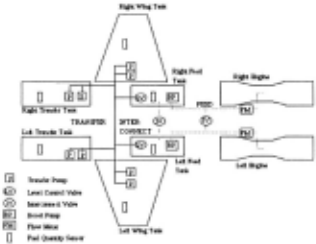
Figure 1 illustrates the fuel transfer system that we use for our experiments. The fuel system is designed to pro vide an uninterrupted supply of fuel at a constant rate to the aircraft engines, and at the same time to maintain the center of gravity of the aircraft. The system is symmetri cally divided into the left and right parts (top and bottom in the schematic). The four supply tanks (Left Wing (LWT), Right Wing (RWT), Left Transfer (LTT), and Right Transfer (RTT)) are full initially. During engine operation, fuel is transferred from the supply tanks to the receiving tanks (Left Feed (LFT) and Right Feed (RFT)) based on a pre-defined sequence. The fuel transfer se quence is controlled by valves on pipes at the outlet of the supply tanks and the inlet to the feed tanks. The hy brid bond graph segment for the connection between a wing tank and a feed tank, shown in Figure 2, illustrates the component-oriented modeling approach for the HBG. An element called switching implements the finite state automata discussed earlier. The HBG framework also associates one or more parameters with system compo nents. We exploit this in defining a component-based diagnosis methodology, where faults in components are represented as deviations in their parameter values. For example, there are six potential fault candidates in the fuel transfer subsystem in Figure 2. (Pump, Efficiency, Wing Tank, Pipe, Switched, and Feed). In earlier work, we have shown the equivalence between the HBG framework and the hybrid automata representation [16).
2.3 Alternate Model Representations
The bond graph can be used to systematically derive al ternate model representations. Three representations are used to solve different sub-tasks in the diagnosis scheme: (i) state space equations, for tracking of continuous be havior, (ii) temporal causal graphs for qualitative fault isolation, and (iii) input output equations, for parameter estimation and refinement of the fault isolation results. A
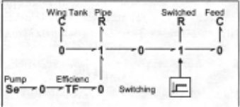
detailed description of temporal causal graphs (TCG) can be found in[ 14, 15] and is not repeated here. Essentially the TCG captures causal and temporal relations between variables in the system. The vertices in the graph repre sent variables of the system and the edges (with labels) represent the types of relations between the variables.
3 MBD Architecture
Our diagnosis architecture implements a scheme to track the nominal system dynamics using an observer that is robust to model uncertainties and noise in the measure ments. It uses a fault detection scheme to trigger the fault isolation scheme when discrepancies are detected be tween the observed and predicted measurements, tracks and analyzes the fault transients using fault signatures to isolate_ the .fault, and then employs a quantitative parame ter estimatiOn scheme to determine the magnitude of the fault. Our work focuses on component parameter faults which are multiplicative, i.e., faults directly affect th~ system dynamics models. As discussed earlier, the hybrid n_ature of the system complicates the tracking and diagno SIS tasks, because mode transitions cause model switch ing, which has to be included in the online behavior tracking and fault isolation algorithms. For pragmatic reasons we simplify our algorithms by making the single fault assumption.
We have developed a novel approach that combines qualitative and quantitative algorithms for fault isolation. This extends our earlier work [ 12] on fault isolation in continuous systems. The qualitative approach overcomes limitations of quantitative schemes, such as convergence and accuracy problems in dealing with complex non linearities and lack of precision of parameter values in system models. It plays a significant role in cutting down on computational complexity, enabling online algorithms for fault isolation in the hybrid framework. The qualita tive reasoning scheme is fast and effective, but it has lim ited discriminatory ability. To uniquely identify the true fault candidate, we employ a quantitative parameter esti mation scheme, which also returns the magnitude of the deviated parameter.
3.1 Tracking and Fault Detection
Our hybrid observer is implemented as a combination of an extended Kalman filter (EKF) and a hybrid automaton to track continuous behavior in individual modes of op eration, and discrete mode changes (controlled and autonomous), respectively. At mode changes, the new state space model and the initial state of the system are recomputed. Model uncertainty and measurement noise are implemented as white, uncorrelated Gaussian distri butions with zero mean. The state space model in mode q is defined as:
where w is distributed N(O,Q) and vis distributed N(O,R), and Q and R are process and measurement noise covariance matrices. It is assumed that wk incorporates the Nq.Xk term that captures modeling errors in the system. In our work, the Q and R matrices were determined em pirically. The extended Kalman filter algorithm follows the methodology presented in [ 4].
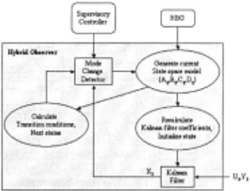
Mode change calculations are based on the system mode at time step k, qk. and the continuous state of the system, Xk. The discrete controller signals to the plant are assumed known. For controlled transitions, we assume such a signal is input at time step k, and the appropriate mode transition is made at time step k+ 1 to q k+ I· For autonomous transitions, the estimated state vector, xk is used to compute the Boolean functions that signal mode tr~nsitions .. Note that several transition functions may be tnggered simultaneously. They are combined to derive the new system mode. A mode transition results in a new state equation mode~, i.e., the matrices Fq, Gq, Cq, and Dq are recalculated onlme. We have developed an efficient symbolic solver that can construct state equation models from equation fragments. The equation fragments corre spond to constituent equations defining component be havior, and the junction relations. When switching oc curs, sets of equation fragments are de-activated, and others are activated. The new state equations are then derived incrementally. To simplify analysis, we assume that mode changes and faults occur only after the Kalman filter state estimate has converged to its optimal behav ior. Further details of the observer implementation are presented in [15].
Fault detection is performed by first computing esti mates of the output variables Yk from the state estimates Xk· We then compute a smoothed estimate Yk using an FIR filter. Finally we compute the residual (Yk-ok), where ok are the observations at time step k. If this residual rk is above a threshold E for a pre-defined number of time steps, then a fault is signaled.
3.2 Fault Isolation and Identification
Once a fault has been detected, fault isolation and identi fication is performed to uniquely isolate the fault and determine its magnitude. Our fault isolation and identifi cation architecture is presented in Figure 4 involves three steps: (i) qualitative roll-back, (ii) qualitative roll forward, and (iii) quantitative parameter estimation.
For hybrid systems, discontinuous changes in meas ured variables can only occur at the point of failure or at points at which discrete mode changes occur in the plant behavior. At all other time points the plant behavior is continuously differentiable. We take advantage of this fact for qualitative analyses of all measured variables, Yk· The residual (rk) for any variable is defined as the differ ence between the measure plant output and the nominal expected plant output. Since both of these are continu ously differentiable after the fault occurrence, and after each mode change, the residual can be approximated by the Taylor series expansion:
We can then represent the residual as the coefficients of the magnitude and higher order derivative terms of the residual. Instead of representing them in quantitative form, qualitative values (-, 0, and +) are used to indicate if the coefficient is below, at, or above zero.
The qualitative analyses that comprise of the roll-back and roll-forward steps work on these qualitative coeffi cients. After detection of the fault, the signal to symbol generator is responsible for converting the measured ob servations to symbolic form at each time step. The dis cussion of the computation of the residual and the con verting it to symbolic form is presented in [11], and not repeated here.
The roll-back algorithm can be summarized as follows . Given the observer estimated mode trajectory Q = {q ~>q2, .. . , qk}, we first use the back propagation algorithm [14) to generate hypotheses in mode qk. The deviated symbols at the time of fault detection (a) are back propagated through the temporal causal graph in mode qk to identify causes for the deviations. Since the fault may have oc curred in previous modes, we then go back in the mode trajectory and create hypotheses in each of the previous modes qk-J, qk-2· ... , qk-n+J, where n is a number deter mined externally by diagnosability studies. During the crossover from a mode to a previous mode, the symbols need to be propagated back across the mode change. This is done by using the inverse of the reset functions (f 1 ) associated with the mode transition. For example, the symbols to be propagated in mode qk-I is obtained as f 1 (a,q~o qk-J) . The hybrid hypotheses generation algorithm returns a hypotheses set, H = {h1, h2, ··· , hm}, where each hypothesis h; is a three-tuple {q,p) .. }, where q represents the mode in which the fault is hypothesized to have oc curred, p is the parameter whose deviation corresponds to the fault, A is the direction of deviation of parameter p.
The occurrence of the fault may change the parameters of the functions that determine autonomous transitions leading the observer to incorrectly predict (or not predict) an autonomous transition. Hence the current mode esti mated by the hybrid observer may not be the actual mode of system under hypothesized fault conditions. We need to estimate the current mode of the system for each hy pothesis. However, we still do not have the quantitative value for the faulty parameter, implying that we cannot accurately determine the current mode of the system. To solve this problem we take advantage of the fact that the same sequence of mode transitions in any order would lead the system to the same end state. This follows from the fact that each mode transition essentially changes the status of a switched junction in the hybrid bond graph representation. Based on this observation, for each hy pothesis, we apply all controlled transitions (assuming that no autonomous transitions have occurred) that have occurred since the hypothesized fault mode to get an es timated current mode. This is known as the roll-forward process.
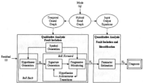
We can now use the model (TCG) to predict the ex pected qualitative values for the residuals (signatures) in the current estimated mode for each hypothesis. This is done through a forward propagation algorithm [14). The fault hypotheses in the estimated current mode are com pared with the symbols generated by the signal to symbol generator using a progressive monitoring scheme [14]. If there is a mismatch, the hypothesis cannot be dropped immediately, we assume that an autonomous mode transi tion may have caused this mismatch. We apply all possi ble autonomous transitions to the current estimated mode and derive m new estimated current modes for the hy pothesis, where m is the number of possible autonomous transitions. For each of these m new modes, we can gen erate the qualitative signature using forward propagation and compare this against observations. In case of mis match we hypothesize occurrence more autonomous tran sitions and repeat the process. Once the total number of transitions (controlled + hypothesized autonomous) ex ceeds the diagnosability limit, further mismatches in sig natures and symbols eliminate hypotheses.
In other work [12], we have shown the limited dis criminatory capabilities of the qualitative progressive monitoring scheme. This often leads to multiple fault hypotheses being reported as the diagnostic result. Even when we are left with only one hypothesis, determining the magnitude of the parameter associated with the hy pothesis is essential to continue tracking the plant behav ior in the faulty situation. We use a parameter estimation technique based on the least-squares estimation method for further fault isolation and identification. Applying a statistical hypothesis testing scheme to the error in the fault identification task leads to unique fault isolation, and an estimate of the deviated parameter value. Con sider the input output equation form:
where U are the inputs, Yare the outputs, a's and b's are constant coefficients and q is the forward delay operator. The typical parameter estimation task is to estimate the a's and b's using measurements, u and y. The optimal estimate is given by: Best = (ai t:Pl 1 cprz, where ()is avec tor of a's and b's, <l> is the regression vector, and Z is current output vector. The single fault assumption im plies that only one parameter in unknown. So, for each remaining hypothesis, we rewrite () in terms of the corre sponding hypothesized fault parameter p. If we assume a first order polynomial relation (it is possible to extend this to arbitrary polynomial relations): () = K1p+K0, where K1 and K0 are matrix constants. Now we can re formulate the estimation problem and obtain the optimal estimate for f as:
| Time | Measured Deviation | Fault Set |
|---|---|---|
| 433 | Transfer Manifold Pressure (XMP} | 13 fault candidates |
| 434 | XMP: discontinuous I 0 candidates | |
| 439 465 | Mode Change: Left Feed Tank On Mode ChanRe: Left Feed Tank orr | |
| 469 | LeftWing Tank Pres- sure++ | LWT_Pipe.R + LeftWingTank.TF- LeftWingTank.R + Leg26.R- |
| 471 | Mode ChanRe: Left WinR Tank - Second Pump On | |
| 489 | Left Feed Tank Pressure-- | LWT_Pipe.R + LeftWingTank.TF- LeftWingTank.R + |
| 528 | Mode ChanRe: Left Feed Tank On | |
| 528 | Parameter estimation started | LeftWingTank. TF fault coefficient: 0.658041 |
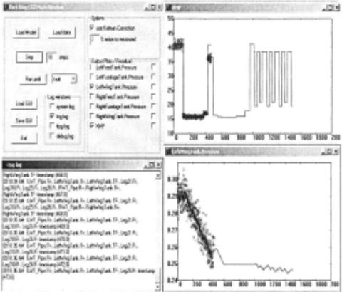
For each remaining hypothesis, we compute the input output equations of the system in the estimated current mode from the bond graph. This can be achieved by computing the temporal causal graph from the bond graph. The TCG can then be used to compute the signal flow graph, which can be used to derive the input output equations. Please note that the signal flow graph still contains parameters in symbolic form as opposed to ac tual numeric values. This gives us a parameterized input output equation. We then calculate the K1 and K0 matri ces. Finally we accumulate u andy values, and estimate p using the above expression. This may also be used for fault isolation by plugging back the estimated parameter in the state space equations and computing the predicted values for the outputs. Hypotheses whose predicted out put values are statistically different from actual output values are eliminated. Table I illustrates an experimental run for a left wing tank pump degradation (33% loss) at time step 150. The initial change was observed in the transfer manifold pressure at time step = 433 (Fig. 5), but two mode changes occurred between the fault occurrence and its detection. The roll back process was employed, and this produced an initial list of 13 candidates. Detect ing that the transfer manifold pressure was discontinuous reduced the candidate set to I 0 faults. As other measure ments deviated over time (first left wing tank pressure, then left feed tank pressure), the candidate set was fur ther refined. Mode changes required the re-derivation of the system models, and the computation of new signa tures to track system behavior. The qualitative scheme reduced the candidate set to 4, and then the parameter estimation scheme was invoked. This resulted in generat ing the correct fault hypothesis, and a correct estimation of the faulty parameter.
4 Experimental Results
We demonstrate the effectiveness of our diagnosis scheme on a real world example, the fuel system of fighter aircraft (Fig. 1 ). The pumps are modeled as a source of effort (pressure) with a transformation factor that defines its efficiency. The pipes are modeled as nonlinear resistances.
The diagnosis experiments used a controller sequence provided by Boeing. The performance of the hybrid ob server in tracking the nominal data (with 3% noise) through mode transfers is illustrated in Figure 5 for the transfer manifold and left wing tank pressure measure ments. The dots represent the measured data and the black line shows the observer estimates. A number of diagnosis experiments were run for different noise values and fault magnitudes (see [15] for details) .
| WTP | WTR | TTP | TTR | SPR | FTP | FTR | |
|---|---|---|---|---|---|---|---|
| WTP | - | X | ..; | ..; | ..; | ..; | ..; |
| WTR | X | - | ..; | ..; | ..; | ..; | ..; |
| TTP | ..; | ..; | - | X | ..; | ..; | ..; |
| TTR | ..; | ..; | X | - | ..; | ..; | ..; |
| SPR | ..; | ..; | ..; | ..; | - | ..; | ..; |
| FTP | ..; | ..; | ..; | ..; | ..; | - | X |
| FTR | ..; | ..; | ..; | ..; | ..; | X | - |
Table 2 summarizes the different fault classes that can be distinguished by our diagnosis algorithms. The fault classes are as follows: (i) Wing Tank Pump (WTP), (ii) Wing Tank Resistance (WTR), (iii) Fuselage Tank Pump (TTP), (iv) Fuselage Tank Resistance (TTR), (v) Switched Pipe Resistance (SPR), (vi) Feed Tank Pump (FTP), and (vii) Feed Tank Resistance (FTR). The ~ mark in row i and column j indicates that fault class i can be distinguished from fault class j. The x mark indicates that the current controller sequence and set of measure ments are not sufficient to distinguish between the pair in question. From the table, we see that we cannot distin guish between tank pump faults and tank outlet pipe re sistance faults. However, this is true only for a pump ef ficiency (T F-) decrease and pipe resistance increase (R + ). Since the pump efficiency cannot increase (no TF+ fault), pipe resistance decreases, R-, (i.e., leaks) can be uniquely identified. All other classes of faults can be distinguished from one another. In some cases, the isolation may be achieved only after mode changes occur.
5 Summary
In this paper we have presented an integrated approach to solving the tracking, fault detection, isolation, and identification tasks for hybrid systems. The novel contri bution of the presented work is the extension of continu ous system model-based diagnosis techniques to hybrid systems. These include the hybrid observer that combines an extended Kalman filter and hybrid automaton, hybrid fault isolation through roll back and roll forward using qualitative analysis, and the single parameter estimation for further fault isolation and identification. Our work is motivated by the requirements of the fault accommoda tion task, where diagnosis has to be performed online for embedded systems during their operation. Hybrid diagno sis techniques directly apply to embedded systems and else where [15]. We have also demonstrated through time and space complexity analysis that our algorithms can be applied to online analysis in resource constrained envi ronments.
Acknowledgments
The DARPA/IXO SEC program (F30602-96-2-0227), NASA IS NCC 2-1238, and The Boeing Company (Kirby Keller and Tim Bowman) have supported the activities described in this paper. We would like to thank Dr. Ga bor Karsai, Tivadar Szemethy, Nagabhushan Mahadevan, and Eric Manders for their help.
@inproceedings{ijcai2003p56,
  title     = {Model-based Diagnosis of Hybrid Systems},
  author    = {Narasimhan, Sriram and Biswas, Gautam},
  booktitle = {Proceedings of the Eighteenth International Joint Conference on
               Artificial Intelligence, {IJCAI-03}},
  publisher = {International Joint Conferences on Artificial Intelligence},
  editor    = {Georg Gottlob and Toby Walsh},
  pages     = {376--380},
  year      = {2003},
  url       = {https://ijcai.org/proceedings/2003/56},
}
TY - CPAPER TI - Model-based Diagnosis of Hybrid Systems AU - Narasimhan, Sriram AU - Biswas, Gautam T2 - Proceedings of the Eighteenth International Joint Conference on Artificial Intelligence, IJCAI-03 PB - International Joint Conferences on Artificial Intelligence PY - 2003 SP - 376 EP - 380 UR - https://ijcai.org/proceedings/2003/56 ER -Copied
Machine-readable versions of this paper, for tools and AI agents:





