A Formal Modeling Scheme for Continuous Systems: Focus on Diagnosis

1 Introduction

Diagnosis of engineering systems requires finding a com­ ponent or a set of components that are the primary cause for observed discrepancies between normal (predicted) behavior and observed behavior of the system 1 [Davis and Hamscher, 1988]. Model-based diagnosis researchers (e.g., [Davis, 1984]) have successfully developed effective and efficient device-independent diagnosis algorithms that consist of two primary subtasks: (i) candidate gen­ eration, and (ii) measurement selection. However, the availability of appropriate system description models that make all the information required for diagnosis ex­ plicit is the key to the success of this methodology[Davis and Hamscher, 1988]. Most past efforts (especially logic­ based approaches to diagnosis) have focused on dig­ ital circuits[de Kleer and Williams, 1987; Hamscher, 1988] . Whereas diagnosis of complex circuits provide formidable computational challenges[de Kleer, 1991], the problem becomes even more complicated when one tries to apply these methodologies to dynamic continuous sys­ tems. The primary reason for these difficulties can be at­ tributed to the lack of computationally tractable models that are precise enough to be useful for diagnosis[Dague et a/. , 1987; Davis and Hamscher, 1988] .

·Partially supported by grants from Federal Express Cor­ poration and Office of Naval Research (N00014-91-J-1769) .

1 An alternate approach is parameter-oriented diagnosis: correct system malfunctions by appropriate control actions (e.g., [Gallanti et al., 1989]) .

This paper discusses a formal modeling scheme for continuous physical systems, adapted from the bond graph modeling scheme in systems dynamics[Rosenberg and Karnopp, 1983], that generates appropriate system descriptions for efficient component-oriented, logic-based diagnosis. This is achieved by ensuring that: (i) individ­ ual components and component behaviors are explicitly represented, and (ii) relations between measurable pa­ rameters and individual components are readily deriv­ able from the models. Our diagnosis algorithm starts off with a set of equations that link output measurements to component parameters, and generates a partial conflict set by performing qualitative causal analysis on these output equations . The partial conflict set forms the ba­ sis for efficient candidate generation and measurement selection algorithms.

Adopting this modeling framework provides a unifying framework for studying diagnosis of both continuous and discrete (digital) systems. Our focus in this paper is on modeling for diagnosis. This involves generation of the system description as a set of equations that relate mea­ surements to system components and converting them to partial conflict sets. Candidate generation and mea­ surement selection are discussed in detail elsewhere[Yu and Biswas, 1992]. To illustrate our methodology, we de­ velop diagnosis models of the pneumatic system of DC10 aircraft . This system regulates air pressure and tem­ perature drawn from a jet engine before it is delivered through the manifold system to different subsystems of the aircraft that constitute loads (e.g., the wing de-icing system) . The pneumatic pressure is regulated by a pres­ sure regulator, and the temperature is controlled by a precooler subsystem( see Fig. 1) .

2 From Physical Schematics to Bond Graph Models

Effective problem solving using model-based approaches requires the ability to dynamically construct models of a system that are both parsimonious and adequate for the specific task[Falkenhainer and Forbus, 1992; N a yak et a/., 1992]. The overall modeling method ts more elaborately described as a four step process:

1. decomposition into primary mechanisms,

1. model fragment selection based on mechanisms and assumption classes; composition of fragments to generate the overall model,
2. output equation generation, and
3. partial conflict generation from measurements using qualitative causal analysis.

Formally, the model construction problem is: Given: (a) A schematic descriptionS that includes com­ ponents of the system and their interconnections, and a functional description F that defines the expected behav­ IOrs,

• (b) A domain theory Th consisting of a set of model frag­ ments represented as bond graphs or bond graph com­ ponents and a set of rules that determine their use. Each model fragment represents a mechanism, and
• (c) A task description T that defines the task to be ac­ complished (e.g., diagnosis) and the level of detail in which this task needs to be performed (for diagnosis this is the list of possible diagnostic candidates)

Produce: A bond graph model of the overall system for deriving its behavior. Since our focus is on diagnosis, it is also important that given adequate measurements any fault among components (specified by T) should be identifiable.

In our modeling scheme, individual bond graphs usu­ ally correspond to different physical domains of system behavior, such as thermodynamics and fluid mechanics. Therefore, the bond graph model of a system may be made up of a number of individual bond graphs.

2.1 Bond Graphs as a Modeling Language

The bond graph methodology[Rosenberg and Karnopp , 1983] provides a formal and systemati c language for modeling dynamic systems that make a number of as­ sumptions and issues about system functionality explicit . Bond graphs are highly organized domain independent structures that are based on a small number of primitive elements: resistances or dissipators (R), energy storage elements (capacitors C and inertial elements I), ideal sources of effort S, and flow S1 , and transformational elements (transformer T F and gyrator GY). These el­ ements take on different physical forms in different do­ mains, but interactions between them are expressed in a domain independent way: as energy transfers repre­ sented as directed bonds. Each bond has an associated effort and a flow variable, where effort x flow= power , the rate of energy transfer. Examples of effort and flow variables are temperature and heat flow rate in thermo­ dynamics and force and velocity in mechanics. Connec­ tions between elements are established by common flow (series) or !-junctions, and common effort (parallel) or 0-junctions.

There exists a systematic procedure for building bond graph models of physical systems[Rosenberg and Karnopp, 1983]. Fig. 2 illustrates the bond graph model of a simple heat exchanger mechanism, which de­ picts heat flow through a resistive junction R between two materials represented as capacitances C1 and C2 . This representation is not unlike the view-process struc­ ture, the fundamental basis for modeling in the QPT

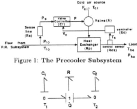
framework[Forbus, 1984] . The R el.ement models the relationship between heat flow rate Q and temperature difference T1 - T2 . If T1 - T2 is not large R-Q = Tt - T2 . The C elements are thermal capacitances which repre­ sent the thermal energy stored in an amount of material as a function of the temperature of the material, i.e. , ilQ · C = ilT.

Primitive bond graph elements , such as resistors and capacitors represent mechanisms [Top and Akkermans, 1991] which may or may not be in 1-1 correspondence with individual system components. To extend this framework for component-oriented diagnosis, individ­ ual components related to measurable parameters are represented explicitly by creating component and co­ component parameters.

Component parameters directly relate to the function­ ality of components under diagnostic scrutiny, e.g., R (resistance) directly relates to a primary functionality of a heat exchanger component. A component defini­ tion may include multiple component parameters that represent different aspects of component functionality. Component parameter definitions also include its Possi­ ble Directions of Change (PDC) . This is characteristic of specific components, e.g., some resistance values only increase as a system degrades. The PDC of a compo­ nent parameter takes on one of three values: + (only increases) , - (only decreases), and? (can change in ei­ ther direction) . It determines how that parameter and hence the corresponding component can affect output parameters. This information helps narrow down possi­ ble candidates for diagnosis.

Co-component parameters are not directly associated with primitive component functionality. They represent bond graph elements that are introduced to complete system functionality description. The thermal capaci­ tances of the heat exchanger (Fig. 2) in the precooler sys­ tem (Fig. 1) are not individual components. They model the air masses that exchange heat . The air masses are in turn related to flow rates of the incoming air streams. Thus , co-component parameters are defined in terms of other component parameters.

In addition, the model defines input variables associ­ ated with source elements of the bond graph. They are exogenous to the system being analyzed. Output vari­ ables represent values which can be measured as part of the observation set. Characterization of parameters depend on the viewpoint in which we analyze a system. Parameters that are known to be insignificant or un­ changed for a specific diagnostic task are considered to be constant. Parameters that express interactions be­ tween the system and other subsystems not modeled are also considered constant (because: their effects are con­ sidered to be exogenous to the di ~gnostic situation).

For the pneumatic system, jet engine pressure and temperature are input variables. Possible output or mea­ surable parameters are Pho and Tho, the output pressure and temperature of the bleed air at the load, and Pro the pressure at the pressure regulator output. Resistance at the heat exchanger junction Rp and the resistance of the sense line to liquid flow R,, are examples of component parameters for the precooler subsystem.

2.2 System Decomposition

In general, system decomposition being task- and view­ point dependent is hard to automate. For example, if it is sufficient to determine that the cause of a problem is jet engine failure then the engine can be modeled as an effort source. If the diagnosis task requires that the cause of the problem within the engine be determined, then it is important to model explicitly the internal mecha­ nisms and components that govern engine functionality. We make the assumption that the modeler performs the system decomposition task by selecting the set of pri­ mary mechanisms that define its functionality.

In the bond graph framework , primary mechanisms can be classified as: (i) energy sources, (ii) energy flow and storage mechanisms, and (iii) energy transformation mechanisms. In addition, we define a special class of mechanisms called feedback mechanisms to facilitate the modeling process. Examples of primary mechanisms in the fluid domain are flow sources (e.g., pumps) , fluid storage mechanisms (e.g., tanks and pipes), and flow or transport mechanisms (e.g., pipes).

The modeler begins the decomposition process by first identifying the different domains that describe system behaviors of interest. In the pneumatic system, the do­ mains of interest are: (i) thermal, (ii) fluid, and (iii) me­ chanical. Simultaneously the modeler studies the speci­ fication task T and the system schematics to pick com­ ponents that are of diagnostic interest . This leads to the selection of one or more component parameters that gov­ ern behaviors of interest for each component. The next step involves selection of the primary mechanisms in the bond graph framework. The precooler system (Fig. 1) system is represented as a composition of three mech­ anisms: (i) heat transfer between materials through a resistive junction, (ii) feedback mechanism for tempera­ ture control, and (iii) resistive fluid flow through a valve. Note that the system decomposition step produces pri­ mary mechanisms and their list of associated compo­ nents.

2.3 Modeling with the Bond Graph Library

Once primary mechanisms have been identified, model construction takes on a compositional model­ ing flavor[Falkenhainer and Forbus, 1992; Nayak et a/., 1992], which is implemented as a two steps process: (i) selection of bond graph fragments that are derived from primary mechanisms and assumption classes, and (ii) composition of the fragments to build bond graph mod­ els of the system under consideration. The modeler's task is facilitated by developing bond graph libraries that represent collections of mechanisms in various domains. An example of an element in the library is the heat ex­ changer mechanism fragment (Fig. 2). For each primary mechanism, the modeler's task is to index into the li­ brary and pick the appropriate bond graph fragment(s) that corresponds to this mechanism, and then to map physical system components into this generic structure. In the heat exchanger if heat transfer occurs uniformly across a thin slab of material, the thermal resistance R is a function of the thermal conductivity, the cross­ sectional area, and the thickness of the material. For two blocks of metal, the capacitance C of each block is a function of its mass and specific heat. If the heat ex­ change occurs between two fluids flowing through pipes, the capacitance value computations are more complex.

Given a description of a primary mechanism and its components, how does the modeler index into the bond graph library and pick the appropriate fragment ? We take the approach proposed by [Falkenhainer and For­ bus, 1992] and [Nayak et a/., 1992] to describe an in­ dexing mechanism in terms of assumption classes. An assumption class represents a consistent combination of the physical setting of the system, its operating condi­ tions, and the conditions that influence the behavior of its components. Turbulent incompressible flow through a resistive pipe represents an assumption class. Viscous flow through a pipe with no resistance is inconsistent, and cannot be an assumption class. Assumptions can be further classified into (i) characteristic assumptions, and (ii) component assumptions.

Characteristic assumptions pertain to behavioral con­ straints and assumptions that are global in nature. For fluid flow the following assumptions are relevant:

• compressibility: compressible, incompressible,
• dimensionality: one, two, three dimensional,
• velocity: subsonic, supersonic,
• viscosity: inviscid, viscous, and
• turbulence: laminar, turbulent.

These assumptions are not all independent, and some combinations may be invalid.

Component assumptions define, for each subsystem, properties of its components that need to be explicitly represented in the model. Each property corresponds to a primitive bond graph mechanism. For example, con­ sider a pipe as a fluid flow mechanism. If its storage capacity is important in the analysis, the pipe is mod­ eled as a combination of R and and C elements. If its storage properties are not relevant, the pipe is modeled as a simple resistive element R.

Characteristic and component assumptions are orga­ nized into mutually exclusive assumption classes, which form the basis for indexing into the bond graph library and retrieving appropriate model fragments. A model fragment is a bond graph segment and a set of equa­ tions, that define effort-flow variable relations for indi­ vidual bond-graph elements.

A bond-graph segment may have multiple equations to define its behaviors. Each equation set corresponds to a specific assumption class. For example, pressure drop in a pipe for incompressible laminar flow is represented by the equation: t::..P = ~~~~I'Q, where J1. is the viscosity, I is the length , and d is the inside diameter of the pipe. For turbulent flow, the relation becomes: t::.P = atQIQI~, where at is a constant that is often determined experi­ mentally.

Selected bond graph segments are then composed to build the bond graph model of the system. This difficult task[Biswas et a/. , 1992] is much simplified in the bond graph framework, because interactions between compo­ nents are expressed in one of three domain-independent ways: (i) energy transfers represented as directed bonds, (ii) links between segments established by 0- and !­ junctions, and (iii) interactions between segments in dif­ ferent domains established by TF andGY elements.

The bond graph modeler has been implemented in X window and C with a simple graphics- and menu-based interface[Yu, 1992]. As part of the modeling system, we have developed adequate bond graph libraries in the thermodynamic and fluid domains.

2.4 Bond Graph Model - Precooler Subsystem

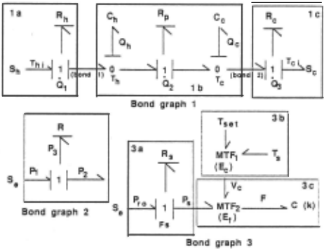
As discussed earlier, the temperature regulating part of the pneumatic system (Fig. 1) is composed of the heat exchanger, the pneumatic flow valve, the feedback con­ trol subsystems. Three primary mechanisms are iden­ tified for the heat exchanger subsystem: the heat ex­ changer mechanism, and two source mechanisms. The bond graph fragment for the heat exchange mechanism (fragment lb, Fig. 3) models uniform heat exchange between the two air masses through a resistive junction Rp. Each mass is represented as a thermal capacitor. Bond graph fragments for the hot and cold sources (fragments Ia and lc) provide heat at constant temperature (Th and Tc) along resistive pathways, i.e., there is heat loss dur­ ing transport of the air mass. The bond graph fragments are then connected using bond 1 and 2 to form the model for the heat exchanger subsystem (bond graph 1, Fig. 3).

Bond graph 2 for the valve subsystem connects the bond graph fragment for resistive flow (model of the valve) with the fragment for an ideal pneumatic source. The amount of pneumatic flow is determined by the re­ sistance in the system, a function of the opening of the valve, which is controlled by the feedback system.

The feedback subsystem has four primary mecha­ nisms: (i) the pneumatic source Se, (ii) resistive flow in the sense line (fragment 3a, Fig. 3), (iii) energy transfor­ mation from temperature difference T,-Tut (T,: sensed temperature, Tut: desired temperature) to a voltage sig­ nal Vc (fragment 3b, Fig. 3), and (iv) energy transfer (fragment 3c, Fig. 3). This bond graph models the physi­ cal situation where the valve controller (MTF2) transfers a fraction of the pneumatic power P, obtained through a sense line (pipe) into a mechanical force F that acts against the valve spring to determine the opening of the valve. The amount of power transferred is determined by a voltage signal Vc from the controller(MTFt).

3 Equation Generation

Output equations that relate output measurements to component parameters are generate in three steps: (i) assign causal strokes to bonds in the bond graph, (ii) generate state equations, and (iii) generate initial output equations and manipulate them algebraically to convert them to the desired form . The first step is discussed elsewhere [Top and Akkermans, 1991] and not repeated here. The algorithms for the second and third steps are presented below. Their implementation makes calls to the Mathematica package, which performs some of the required symbolic and algebraic manipulations.

3.1 State Equation Generation

In the bond graph framework, an nth order system is modeled as a set of n first order differential equations in the following form:

where x; 's are state parameters, i; 's are their deriva­ tives, z; 's are component parameters, Uj 's are input pa­ rameters, g; 's are algebraic functions , and Ck 's are co­ component parameters.

The standardized procedure for generating state equations[Rosenberg and Karnopp, 1983] involves for­ mulation of initial equations associated with the I, R, and C elements. For example, the hot air mass is rep­ resented as a capacitor element satisfies the equation 2 Th = Thi + &- . First order differential equations are then formulated for each state variable. The Qh variable in bond graph 1 can be expressed as: Qh = Q1 - Q2 . Mak­ ing appropriate substitutions using equations for the I, R, and C elements we get:

2 The two air masses are modeled as lumped systems. More detailed piecewise models can also be created.

3.2 Output Equation Generation

The general form of an output equation is:

where YA: is an output parameter. Equation generation is based on the following assumptions: (i) the physical systems we deal with are linear or are modeled by linear approximations, and (ii) the systems was operating nor­ mally in a steady state, and diagnosis is initiated when system parameters deviate from their steady state values (i.e., we perform steady state diagnosis).

For generating output equations in the proper form, assumption (ii) is exploited to set x; to 0 (no change in x;) or a constant (x; changes at a con­ stant rate). The state variables are then solved for and substituted into the output equations to generate: Yi = ff(zl, .. . ,z;,ul , . .. ,ur,cl,· ···cm)· To relate co­ component parameters to component parameters output equations are generated from bond graphs where the co­ component parameters are treated as output parameters. This is repeated till all equations for co-component pa­ rameters are of the form: c; = f:' ( z1 , .. . , z;, u1, . . . , Ur ). The algebraic manipulations and solution of linear equa­ tions are executed using the Mathematica package.

This method applied to the output temperature Tho produces the initial output equation:

Co-component parameters are solved for recursively un­ til they are represented as a function of component and input parameters only. For the pneumatic system, the following set of equations are generated. (Details of their derivation appear in [Yu, 1992].)

A number of these parameters are constants; some are measurable parameters (e.g., Pro) and others are compo­ nent parameters (e.g. , R,). The final form of the output equations may be generated by systematically substitut­ ing for co-component parameters till all parameters in the equations are either input parameters or component parameters. The equations are then in a form where di­ rect relations could be established with component pa­ rameters to generate potential conflicts.

4 Generating Partial Conflicts

For each output variable whose value is known, a partial conflict which depends on the deviation of the measured value is constructed. Partial conflict extends the notion of conflicts[de Kleer and Williams, 1987], which are de­ fined in terms of a set of assumptions (e.g., a component is normal) related to a symptom that produces an incon­ sistency. In their ATMS-based methodology, conflicts were generated incrementally as new measurements are made. Earlier measurement results were combined with a new one to generate an additional conflict. We take a slightly different but equivalent approach and intro­ duce the concept of a partial conflict. A partial conflict, associated with a measurement, takes one of two forms:

1. if the measurement is deviant, the partial conflict is defined as a disjunction of PDC's for component parameters that are consistent with the direction of change of the measured value, indicating that at least one of them must be deviant in that indicated direction, and
2. if the measurement is within its normal range, the partial conflict is basically a disjunction of a list of component pairs. Each pair represents component parameters that are both normal, or both faulty so that their combined effect on the output parameter is null . (We assume that the normal range of a parameter during steady state operation is given as part of the system description.)

The first step in partial conflict generation analyzes how each candidate component parameter may be linked to the output variable. For example, it may be de­ termined that an increase in the value of a particu­ lar component parameter will cause the output to de­ crease if there are no other changes in the system. To perform this analysis, consider equations each output variable Yk. For each such equation, generate the par­ tial derivative ~, where z; is a component parame­ ter, and compute its qualitative value ( +, -, 0, or ?). Then compute P DC(y, z; +) and P DC(y, z;-) using: P DC(y, zi) = P DC(z;) *~.where* is qualitative mul­ tiplication .

For co-component parameters this analysis is repeated recursively, till direct relations are established between the output variable and component parameters. For ex­ ample, to obtain the relation between R, and Thj.' equa­ tion (2) is first evaluated to produce: if, = -~ E = -, because the qualitative values (A], (k], [E], and (F,] are known to be+. Since X is not an output parameter, the process repeats through equations 4-8, and we get ~~: = -, i.e., if R, increases Tho must decrease.

After relationship between component parameters and output parameters are established, the current set of conflicts are generated: (a) for each deviant parameter y, select all z; 's such that P DC(y, z;) is consistent with the current observed deviation in y; (b) for each nor­ mal parameter y, generate: ( -.z; 1\ .. . I\ -.zn) V ( z1 1\ z2) V ... V ( Zn-1 1\ Zn ), where for each pair (z;, Zj ), P DC(y, z;) and P DC(y, Zj) are complementary and z; :j: Zj is gen­ erated. (PDC's are complementary if one is consistent with + and the other is consistent with - ).

Suppose the observed deviation for Tho is + (above­ normal), a conflict for Tho is generated by analyzing P DC(Tho, z) for each component parameter z. For ex­ ample, if P DC(Tho, R.-) = - the conflict for Tho is: F(Tho) = Rp + V EJ +VI<- V R,- V Ec - v Rc,-· Simi­ larly, the conflict for a normal parameter Pho (the pres­ sure at the output of the pneumatic system) is generated as: F(Pho) = (-.I<p/\-.Rp/\-.Ep/\-.Rpt)V(I(p+/\Ep+) . .. Each z;, -,z; implies (-.z; + f\-,z;- ) . For example, -,J(P represents ( -,]{ P + 1\ -,J( P-). Combining the two partial conflicts F(Tho) 1\ F( Pho) produces the current set of possible candidates. Details of the rest of the diagnosis algorithm appear in [Yu and Biswas, 1992] .

5 Summary

This paper discusses a compositional modeling approach that exploits formal properties of the bond graph mod­ eling language to build models of complex continuous­ valued physical systems. Our overall modeling philos­ ophy mirrors the compositional modelin~ approach pre­ sented by [Falkenhainer and Forbus, 1992j and [Nayak et a/., 1992j. The primary difference is that the more formal properties of the bond graph language allow us to better characterize and formalize the system decomposition and model composition tasks. Besides, bond graph compo­ nents are grounded in physical reality, therefore, models formed by composing bond graph models are guaranteed to be meaningful and physically realizable. The accuracy of the model can be linked to the explicit assumptions that have to be made in linking system mechanisms to bond graph components.

To focus on diagnosis, we demonstrate how partial conflicts are generated from analytic bond graph mod­ els. This leads to efficient candidate generation and mea­ surement selection techniques[Yu and Biswas, 1992]. We have also shown that starting with an analytic equation­ oriented model successively more precise information (such as orders of magnitude information, and quanti­ tative values for parameters) can be introduced , if avail­ able, to derive more accurate diagnostic results . This, as well as our focus on diagnosis, possibly differenti­ ates our work from other bond graph applications in model based reasoning (e.g., Top and Ackermans[Top and Akkermans, 1991]).

To demonstrate the general capabilities of our mod­ eling and diagnosis methodology in handling complex continuous-valued systems, we are currently expanding and refining the bond graph libraries to accommodate the space station thermal bus system. We have reused a number of models created for the pneumatic system, and a number of new mechanisms have also been cre­ ated, e.g., heat exchangers that involve materials in two phases (liquid and vapor). We are also developing con­ trol structures for automated model switching to accom­ modate situations. where changes in operating conditions of the physical system are drastic enough to require dy­ namic changes of bond graph models of the system.