
Phase Transitions of the Asymmetric Traveling Salesman
Proceedings of the Eighteenth International Joint Conference on Artificial Intelligence. Pages 1202-1209.
© 2003 International Joint Conferences on Artificial Intelligence
Abstract
We empirically study phase transitions of the asymmetric Traveling Salesman. Using random instances of up to 1,500 cities, we show that many properties of the problem, including the backbone and optimal tour cost, experience sharp transitions as the precision of intercity distances increases across a critical value. We also show that the average computational cost of the well-known branch-and-bound subtour elimination algorithm for the problem also exhibits a threshold behavior, transitioning from easy to difficult as the distance precision increases. These results provide strong positive evidences to a decade-long open question regarding the existence of phase transitions of the Traveling Salesman.
- E. Balas and P. Toth. Branch and bound methods. In The Trav- eling Salesman Problem, pages 361-401.
- M. N . Barber. Finite-size scaling. In Phase Transitions and Critical Phenomena, volume 8, pages 145-266. 1983.
- M. Bellmore and J. C. Malone. Pathology of traveling-salesman subtour-elimination algorithms. Operations Research, 19:278- 307, 1971.
- C. Borgs, J. T. Chayes, and B. Pittel. Phase transition and finite- size scaling for the integer partitioning problem. Random Struc- tures and Algorithms, 19:247-288, 2001.
- G. Carpaneto, M. Dell'Amico, and P. Toth. Exact solution of large-scale, asymmetric Traveling Salesman Problems. ACM Trans. on Mathematical Software, 21 :394-409, 1995.
- G . Carpaneto and P. Toth. Some new branching and bounding criteria for the asymmetric traveling salesman problem. Man- agement Science, 26:736-743, 1980.
- P. Cheeseman, B . Kanefsky, and W. M . Taylor. Where the really hard problems are. In Proc. JJCAI-91, pages 331 -337. SATlSFlABl LITY IJCAI
- D. Coppersmith and G. B. Sorkin. Constructive bounds and ex- act expectations for the random assignment problem. Random Structures and Algorithms, 15 :113-144, 1999.
- A. Frieze, R. M . Karp, and B . Reed. When is the assign- ment bound asymptotically tight for th e asymmetric traveling- salesman problem? In Proc. of Integer Programming and Com- binatorial Optimization, pages 453-461 , 1992.
- A. Frieze and G. B. Sorkin. The probabili stic relationship be- tween the assignment and asymmetric trave ling salesman prob- lems. In Proc. ofSODA-01, pages 652-660, 2001.
- I. Gent and T. Walsh. The TSP phase transition . Artificial Intel- ligence, 88:349-358, 1996.
- C. P. Gomes, T. Hogg, T. Walsh, and W. Zhang. IJCAI- 2001 tutorial: Phase transitions and stru cture in combinatorial problems. http ://www. cs.wustl . edu/~zhang/links/ijcai-phase transitions.html. Link
- G. Gutin and A. P. Punnen, editors. The Traveling Salesman Problem and Its Variations . Kluwer Academic Publishers, 2002.
- D. S. Johnson, G. Gutin, L.A. McGeoch, A. Yeo, W. Zhang, and A. Zverovich. Experimental analysis of heuristics for the ATSP. In G. Gutin and A. Punnen, editors, Th e Traveling Salesman Problem and its Variations , pages 445-488 . 2002.
- R . M. Karp and J. Pearl. Searching for an optimal path in a tree with random costs. Artificial Intelligence, 21 :99-11 7, 1983 .
- R. M. Karp and J. M . Steele. Probabilistic analysis of heuristics. In Th e Traveling Salesman Problem, pages 181 -205 . 1985.
- S. Kirkpatrick and G. Toulouse. Configuration space analysis of traveling salesman problems. Journale de Physique, 46:1277- 1292, 1985.
- E. L. Lawler, J. K. Lenstra, A. H . G. Rinnooy Kan, and D. B. Shmoys, editors. The Traveling Salesman Problem. John Wiley & Sons, Essex, England, 1985 .
- S. Martello and P. Toth. Linear assignment problems. Annals of Discrete Math ematics, 31 :259-282, 1987.
- C. J. H. McDiarmid. Probabilistic analysis of tree search. In Disorder in Physical Systems, pages 249-260. 1990.
- D. Mitchell , B. Selman, and H . Levesque. Hard and easy di stri- butions of SAT problems. In Proc. AAA1-92, 1992.
- R. Monasson, R. Zecchina, S. Kirkpatrick, B. Selman, and L. Troyansky. Determining computational complexity from characteristic 'phase transitions'. Nature, 400: 133-137, 1999.
- J. Slaney and T. Walsh. Backbones in optimization and approx- imation. In Proc. JJCAI-0 1, pages 254-259, 200 I. IJCAI
- W. Zhang. Phase transitions and backbones of3-SAT and Max- imum 3-SAT. In Proc. CP-2001 , pages 153-167,2001.
- W. Zhang and R. E. Korf. Performance of linear-space search algorithms. Artificial Intelligence, 79:241 -292, 1995.
- W. Zhang and R . E. Korf. A study of complexity transitions on the asymmetric Traveling Salesman Problem. Artificial Intelli- gence, 81 :223-239, 1996.
References were extracted automatically from the PDF and may contain errors.
Full text extracted automatically from the PDF; figures, tables and equations may differ. The PDF is the version of record.
1 Introduction
Phase transition refers to such a phenomenon of a system in which some global properties change rapidly and dramatically when a control parameter crosses a critical value. A sim ple example of phase transition is water changing from the liquid phase to the solid phase when the temperature drops below the freezing point. Phase transitions of combinato rial problems and threshold behavior of combinatorial algo rithms have drawn much attention in recent years [12]. It has been shown that many combinatorial decision problems have phase transitions, such as Boolean satisfiability [7; 21; 22], graph coloring [7] and number partitioning [4].
Another useful concept for characterizing combinatorial problems is that of backbones [ 17; 22]. A backbone variable refers to such a variable that has a fixed value in all solutions of a problem. All such backbone variables are collectively re ferred to as the backbone of the problem. The fraction of back bone, the percentage of variables in the backbone, reflects the constrainedness of the problem and directly affects an algo rithm searching for a solution. The larger the backbone, the more tightly constrained the problem becomes.
*This research was supported in part by NSF grants IIS-0196057 and ITR/EIA-0113618, and in part by DARPA Cooperative Agree ments F30602-00-2-0531 and F33615-01-C-1897. Thanks to Sharlee Climer for the joint work on an algorithm for finding backbones and Alan Frieze for a question on a bin-ball problem. Thanks also to Sharlee Climer, David Johnson, Scott Kirkpatrick and the anonymous reviewers for very helpful comments and suggestions to early versions of the paper.
In contrast to numerous phase-transition studies on decision problems, the research on the phase transitions and backbones of optimization problems is limited. An early work on the symmetric Traveling Salesman Problem, which is an optimiza tion problem, introduced the concept of backbones and left an open question of whether there exists a phase transition o~ the TSP [17]. However, this question has not be addressed smce 1985. One of the most rigorous phase-transition results was obtained on number partitioning [ 4], an optimization problem. However, the phase transition analyzed was the existence of a perfect partition of a set of integers, which is in essence a de cision problem. In our early work, we studied the relationship between the phase transitions of satisfiability, a decision prob lem, and maximum satisfiability, an optimization problem [24]. In addition, the relationship between backbones and average case algorithmic complexity has also been considered [23].
In this paper, we study the phase transitions of the asym metric Traveling Salesman Problem (TSP), which has many real-world applications such as scheduling and routing. The TSP [13; 18] is an architypical combinatorial optimization problem, and also very often a touchstone for combinatorial algorithms. In this paper, we consider the asymmetric TSP (ATSP), where the distance from one city to another rna~ not be necessarily the same as the distance in the reverse direc tion. The ATSP is more general and difficult than the symmet ric TSP (STSP). Our results provide strong positive evidences to the long-standing open question of [ 17] using the more gen eral form of the problem. Another reason that we choose the ATSP rather than the symmetric TSP is that many properties of the assignment problem [19], a problem closely related to the ATSP, are known (Section 3.2) and useful to our analysis.
Specifically, using random problem instances of up to 1,500 cities, we empirically reveal that the average optimal tour length, the accuracy of the best cost function (the assignment problem), and the backbone of the ATSP undergo sharp phase transitions. The control parameter is the precision of inter city distances which is typically represented by the number of digits for the distances. Note that these results are algo rithm independent and properties of the problem. Further more, we show that the average computational cost of the well known branch-and-bound subtour elimination algorithm [I; 3] for the ATSP exhibits a threshold behavior, in which the computational cost grows abruptly and dramatically as the dis tance precision increases.
Two related results are worth mentioning. The research in [26] revealed that the average complexity of the subtour elimination algorithm for the ATSP is controlled by the number of distinct intercity distances. We will further extend this result in Section 5. However, these results are algorithm specific, which may not necessarily reflect intrinsic features of the underly ing problem. The research in [11] studied the decision version of the symmetric TSP. Specifically, it analyzed the probabil ity that a tour of length less than a specific value exists for a random symmetric euclidean TSP, showing that the probabil ity has a one-to-zero phase transition as the length of the tar geting tour increases. Note that the phase-transition result in [ 11] does not address the open question of [ 17] which is on the optimization version of the problem.
2 The Problem and Algorithms
Given n cities and a matrix D = (di,j) that defines the dis tances or costs of pairs of cities, the Traveling Salesman Prob lem (TSP) is to find a minimum-cost complete tour visiting each city once. When the cost matrix is asymmetric, i.e., di,j is not necessarily equal to dj,i , the problem is the asymmetric TSP (ATSP), which is more difficult than the STSP, for both optimization and approximation [14].
The branch-and-bound (BnB) subtour elimination algo rithm [I; 3] solves the ATSP using the assignment problem (AP) as a lower-bound cost function. The AP, which can be solved in O(n 3 ), is to assign to each city i another city j with cost equal to distance d;,j, so that the total cost of all such as signments is minimized [19]. If the AP solution happens to be a complete tour, it is also an ATSP solution.
The BnB search takes the ATSP as the root of the state space and solves the AP to the root node. If the AP solution is not a complete tour, decompose it into subproblems by selecting a subtour from the AP solution and generate subproblems by excluding some edges in the subtour to eliminate the subtour. We used the Carpaneto-Toth subtour-elimination heuristic [6] in our implementation, which generates no duplicate subprob lem, so that the search space is a tree. Next, select as the current problem a new subproblem that has been generated but not yet expanded. This process continues until there is no unexpanded problem, or all unexpanded problems have costs greater than or equal to the cost of the best complete tour found so far.
Our algorithm is, in principle, the same as that of [5], which is probably the best known complete algorithm for the ATSP. The main difference between the two is that we use depth-first branch-and-bound (DFBnB), due to its low space requirement, while [5] used best-first search. We further extended our DF BnB algorithm to finding all optimal solutions and backbones.
3 Previous, Related Results
Two previous lines of work influenced this research and helped reveal the properties of the ATSP.
3.1 Phase transitions in tree search
To capture the tree search of the DFBnB algorithm for the ATSP, we first introduce an abstract tree model. An incremen tal tree [15; 20; 25], T(m, d), is a tree with depth d, and inde pendent and identically distributed (i.i.d.) random branching factors with mean m. Edges are assigned costs that are finite and nonnegative i.i.d. variables. The cost of a node is the sum of the edge costs along the path from the root to that node. An edge cost is nothing but the difference between a node cost and the cost of its parent. An optimal goal is a node of minimum cost at depth d. The overall goal is to find an optimal goal node.
Let Po be the probability of a node having the same cost as its parent. The expected number of child nodes of a node that have the same cost as their parent is mp0 . The following results have been proven [ 15; 20; 25]. Let C* be the expected optimal goal cost of T ( m, d) with m > 1. Let N BF s and N DFS be the expected numbers of nodes expanded by best first search and DFBnB, respectively. As d --+ 00, (I) c· I d --+ a1 and NBFS = NnFs = B(a~) almost surely when mpo < 1, where a 1 and a 2 are constants; (2) C* I (log log d) --+ 1 and NBFS = B(d 2 ) and NnFS = O(d 3 ) almost surely when mpo = 1; (3) C* remains bounded by a constant and N BFS = B(d) and NnFs = O(d 2 ) almost surely when mp0 > 1.
The above results mean that the cost of an optimal goal node almost surely undergoes a phase transition from a linear func tion of depth d to a constant when mp0 increases beyond one. Meanwhile, the expected complexity of best-first search and DFBnB changes dramatically from exponential to polynomial in d as mp0 is reduced below one.
3.2 Relationship between AP and ATSP
The assignment problem (AP) cost function and its relationship with the ATSP have been a research interest for a long time [8; 9; 10; 16]. The relationship between the AP cost, AP(D), and the ATSP cost, AT SP(D), has remarkably different char acteristics under different distance distributions of a random matrix D. The AP(D) and ATSP(D) can be the same with a high probability, or they can differ from each other, with a high probability, by a function of n. If the expected number of zeros in a row of D approaches infinity when n --+ oo, AP(D) = AT SP(D) with a probability tending to one [9]. However, if the distances are uniform over [0, 1, · · ·, lcnnJ], AP(D) = AT SP(D) with a probability going to zero, where Cn grows to infinity with n [9]. Indeed, when the entities of Dare uniform over [0, 1], E(ATSP(D) - AP(D)) 2: c0 ln, where co is a positive constant [10].
4 Phase Transitions of the ATSP
The results in the previous section indicate that the quality of the AP function varies significantly, depending on the under lying distance distribution. Precisely, the difference between the AP cost, AP(D), and the ATSP cost, ATSP(D), has two phases, controlled by the number of zero distances in the dis tance matrix D. In one phase, the difference is zero with high probability, while in the other phase, the expectation of the dif ference is a function of the problem size n.
How does the difference between ATSP(D) and AP(D) change phases? Does it have a sharp phase transition, or does it follow a slow process? Do other properties of the ATSP, such as the backbone, also have phase transitions?
The two-phase result on the accuracy of the AP cost func tion discussed in Section 3.2 is in principle consistent with the phase-transition result of incremental random trees in Sec tion 3 .1. The root of the search tree has a cost equal to the AP cost AP(D) to the problem and an optimal goal node has the ATSP tour cost ATSP(D). If we subtract the AP cost to the root from every node in the ATSP search tree, the root node has cost zero and an optimal goal node has cost equal to ATSP(D)- AP(D). When there are a large number of zero distances in D, the AP cost of a child node in a search tree is more likely to be the same as the AP cost of its parent, since AP will tend to use the zero distances. Therefore, it is expected that more nodes in the search tree will have more than one child node having the same cost as their parents. In fact, the concept of zero distances can be extended to minimal-cost distances. If the cost of the minimal distance is known, we can simply subtract it from every distance without affecting the accuracy of the AP function.
4.1 The control parameter
Furthermore, the concept and role of zero and minimal dis tances can be extended to that of equal distances. The AP to a child node is obtained by excluding one arc, and possibly in cluding some arcs, of a subtour of the AP solution to the parent node. With this new restriction, the child AP is then computed by constructing a new augmenting path from the starting point to the end point of the excluded arc [19]. The child and parent AP solutions usually differ by only a relatively small number of arcs. In other words, the child AP solution is derived by replacing some arcs in the parent AP solution. If the numbers of distances of equal values are large, it is more likely that the child AP cost is equal to the parent AP cost. Conversely, when the number of distinct distances is large, it is unlikely the costs of two APs will be the same. When the distances are uniform over [0, 1, · · ·, R- 1], the probability that the child AP cost is equal to the parent AP cost will depend on the range R. If R is small, relative to the problem size n, this probability will be high. In short, for a given problem size, the accuracy of the AP cost function is controlled by the number of distinct distances in matrix D. More precisely, the accuracy of the AP is deter mined by the fraction, denoted as p( n), of distinct distances.
In practice, however, we do not directly control the number or the fraction of distinct distances. In addition to the actual structures of the "layouts" of the cities, the precision of the distances also affects the number of distinct distances. The precision of a number is usually represented by the maximal number of digits allowed for the number. As a result, the num ber of digits for distances is naturally a good choice for the control parameter.
The effect of a given number of digits on the fraction of distinct distances is relative to the problem size n. Consider a matrix D with distances uniformly over {0, 1, 2, · · ·, R- 1 }, where the rangeR is determined by the number of digits b. For a fixed b, the fraction of distinct distances of a larger matrix D is obviously smaller than that of a smaller D. Thus, the control parameter for the fraction p(n, b) of distinct distances must be in the form of b · f ( n), where f ( n) is a rescaling function on the effect of the number of digits.
To find the scaling function f(n), consider the number of distinct distances of matrix D for a given integer range R. The problem of finding the number of distinct distances is equiva lent to the bin-ball problem as follows. We are given M balls and R bins, and asked to place the balls into the bins. Each ball is independently put into one of the bins with an equal probability. We are interested in the fraction of bins that are not empty after all the placements. Here, for asymmetric TSP M = n 2 - n balls correspond to the total number of nondi agonal distances of matrix D, and R bins represent the possi ble integers to be selected from. Since each ball (distance) is thrown independently and uniformly into one of R bins (inte gers), the probability that one bin is not empty after throwing
-4
- 2
0
2
scaled effective number of d1gits
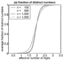
Figure 1: (a) Average fraction of distinct distances in matrix D, p(n, b), controled by the effective number of digits, (J = b log1 0 1 ( n). (b) Average p( n, b) after finite-size scaling. fJo = 2.00195 ± 0.00025 and v = 6.4350 ± 0.0003.
M balls is 1 - (1 - 1/ R)M. The expected number of occu pied bins (distinct distances) is simply R (1- (1- 1/ R)M). Thus, the expected fraction of distinct distances in matrix D is E[p(n,b)] = R(l- (1-1/R)M) /M. NotethatifM ornis fixed, E[p(n, b)] --+ 1 as R--+ oo, since in this case the expec tation of the number of distinct distances approaches M . On the other hand, when R is fixed, E[p(n, b)] --+ 0 when Morn goes to infinity, since all of a finite number of R bins will be oc cupied by an infinite number of balls in this case. We use dec imal values for distances in this paper. Thus R = lOb, where ' b is the number of digits for distances, and we can rewrite E[p(n, b)] as E[p(n, b)] = lOb (1- (1- 1/lOb)M) fM.
It turns out that if we plot p(n, b) against blog1 0 1 (n) , it will have relatively the same scale for different problem sizes n, as shown in Figure 1(a). This means that the scaling function for the effective number of digits is f ( n) = log10 1 ( n). Function b log!l ( n) is thus the effective number of digits that controls the fraction of distinct distances in matrix D, which we denote as (J(n, b) . To have the same effective number of digits f3 on two different problem sizes, say n 1 and n2 with n 1 < n2, the range R should be different. On these two problems, R needs to be nf and ng, respectively, giving nf < ng.
Note that R can also be represented by a number in other bases, such as binary. Which base to use will not affect the results quantitatively, but introduces a constant factor to the results. In fact, since b = log 10 (R), the control parameter (J(n,b) = blog10 1 (n) = logn(R), which is independentofthe base for intercity distances.
Controlled by the effective number of digits b log1 0 1 (n), the fraction of distinct distances p has a phase transition of its own, also shown in Figure 1(a). The larger the problem, the sharper the transition, and there exists a crossover point among the transitions of problems with different sizes. We can examine the phase transitions more closely using finite size scaling. Finite-size scaling [2] is a method that has been successfully applied to phase transitions in similar systems of different sizes. Based on finite-size scaling, around a criti cal parameter (temperature), problems of different sizes tend to be indistinguishable except for a change of scale given by a power law in a characteristic length. Thus, finite-size scaling can help to characterize a phase transition precisely around a critical point of the control parameter as the prob lem scales to infinity. For the problem at hand, the effective
11
~ 0.6
0
~ 04
.1::
~0. 2
~
number of distinct distances f3 = b log!i ( n) and the problem size n play the roles of the temperature and the characteris tic length, respectively. This means that as n goes to infinity, the control parameter becomes ((3 - f30 )n 1 1v, where f3o is the critical point and n 1 1v specifies the change of scale. Using E [p(n,b)] = R (1- (1-1/R)M) /M and numerical meth ods, we obtained the critical value (30 = 2.00195 ± 0.00025 and rescaling component v = 6.4350 ± 0.0003, where the error bounds represent the 95% confidence intervals. The rescaled phase transitions are shown in Figure 1 (b).
Note that the number of digits used for intercity distances is nothing but a measurement of the precision of the distances. The larger the number of digits, the higher the precision be comes. This agrees with the common practice of using more effective digits to gain precision. Therefore, the phase transi tion of the control parameter is in turn determined by the pre cision of intercity distances.
4.2 Phase transitions
With the control parameter, the effective number of digits f3(n, b) for intercity distances, identified, we are now in a po sition to investigate possible phase transitions in (1) the ATSP cost, (2) the probability that an AP cost is equal to the corre sponding ATSP cost, (3) the relative error or accuracy of the AP lower-bound function, and finally (4) the backbone of the ATSP. The answers to the first three problems provides a de tai led picture on the accuracy of the AP cost function, and the answer to the last problem reveals the intrinsic constrainedness among the cities as the precision of distances changes. We ex amine these four problems in turn.
We generated uniformly random problem instances of 100-, 200-, 300- to 1 ,000-cities and 1 ,500-cities. Intercity distances are independently and uniformly chosen from {0, 1, 2, · · ·, R1} for a given range R, which is controlled by the number of digits b. We varied b, with an increment of 0.1, from 1.0 to 6.0 for instances with up to 1,000-cities and from 1.0 to 6.5 for in stances with 1 ,500-cities. For each combination of n and b, we generated 10,000 instances for problems (1)-(3) listed above, and 1,000 instances for problem (4) due to its high computa tional cost. To make the result figures readable, we only use the curves from 100-,500-, 1,000- and 1,500-city problems.
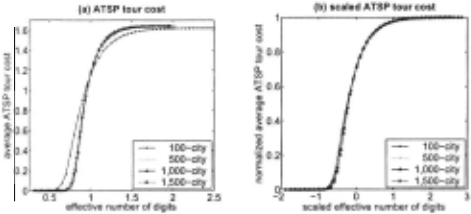
There is a phase transition in the ATSP tour cost, AT SP(D) , shown in Figure 2(a). The reported tour costs are obtained by dividing the integer tour costs from the DFBnB al gorithm by n x ( R - 1), where n is the number of cities and R
the range of intercity costs. Equivalently, an intercity distance was virtually converted to a real value in [0, 1) . By doing this, we can verify the existing analytical result on the AP and ATSP costs. This will be discussed in detail in the next subsection.
As shown, the ATSP tour cost increases abruptly and dra matically as the effective number of digits increases, exhibiting phase transitions. The transitions become sharper as the prob lem becomes larger, and there exist crossover points among curves from different problem sizes. By finite-size scaling, we further determine the critical value of the control parameter at which the phase transitions occur. The scaled result is shown in Figure 2(b ). It is worthwhile to mention that the AP cost (not shown) follows almost the same phase-transition pattern.
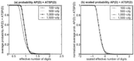
Our numerical results show that when the number of dig its for intercity distances is very small, for example, less than 1.9 digits or R ~ 80 for n = 1, 500, the AP and ATSP costs are equal to zero, meaning that these two costs are the same as well. Given a random distance matrix D, how likely is it that an AP cost will differ from the ATSP tour cost as the effective number of digits f3 increases? We address this question by examining the probability that an AP cost AP(D) is equal to the corresponding ATSP cost ATSP(D) as f3 in creases. Figure 3(a) shows the results, averaged over the same set of instances for Figure 2. As shown, the probability that AP(D) = ATSP(D) also experiences phase transitions. Fig ure 3(b) shows the phase transitions after finite-size scaling.
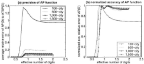
The results in Figure 3 also imply that the quality of the AP function degrades as the effective number of digits f3 increases. The degradation also follows a phase-transition process. This is verified by Figure 4, using the data from the same set of problem instances for the previous two figures.
| n | 1 digits II | AP cost | ATSP cost I | relative AP error(%) |
|---|---|---|---|---|
| 2100 | 8.6810 | 1.6435 ± 0.0008 | 1.6444 ± 0.0008 | 0.0402 ± 0.0009 |
| 2300 | 8.7555 | 1.6439 ± 0.0007 | 1.6445 ± 0.0008 | 0.0368 ± 0.0008 |
| 2500 | 8.8235 | 1.6441 ± 0.0007 | 1.6442 ± 0.0007 | 0.0336 ± 0.0008 |
| 2700 | 8.8861 | 1.6438 ± 0.0007 | 1.6444 ± 0.0007 | 0.0309 ± 0.0007 |
| 2900 | 8.9440 | 1.6439 ± 0.0007 | I .6444 ± 0.0007 | 0.0286 ± 0.0007 |
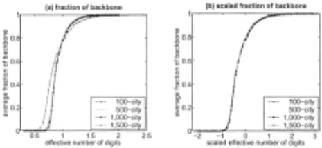
We now turn to the backbone of the ATSP, which is the frac tion of directed arcs that appear in all optimal solutions. The backbones also exhibit phase transitions as the effective num ber of digits for distances increases. The result is included in Figure 5. Interestingly, the phase-transition pattern of the back bone is almost identical to that of the fraction of distinct entities in the distance matrix, shown in Figure I, and that of the ATSP tour cost, shown in Figure 2.
The fraction of backbone captures, in essence, the tightness of the constraints among the cities. As more intercity dis tances become distinct, the number of tours of unique lengths increases. Consequently, the number of optimal solutions de creases and the fraction of backbone grows inversely. When more arcs are part of the backbone, optimal solutions become more restricted and the number of optimal solutions decreases, making it more difficult to find an optimal solution.
4.3 Asymptotic AP precision
As a by-product of the phase-transition results, we now pro vide asymptotic values of the ATSP cost, the AP cost and its accuracy. We attempt to extend the previous theoretical results on the AP cost, which is known to be within (1.51, 1.94) [8], and the observation that the accuracy of the AP lower bounds increases as the problem size increases [1].
We need to be cautious in selecting the number of digits for intercity distances. As discussed earlier, the same number of digits for distances gives rise to different effective numbers of digits on problems of different sizes. Therefore, the number of digits must be scaled properly to have the same effect on prob lems of different sizes when we exam an asymptotic feature.
Therefore, in our experiments, we fixed the scaled effec tive number of digits /3 to a constant. Based on the phase transition of the control parameter in Figure 1, we took /3 = (b log! 0 1 (n) - 2.002)n 1 / 6 .4 35 a constant of 2. /3 = 2 is sufficiently large so that all distances are distinct, regardless of problem size, and the quantities to be examined do not change substantially after finite-size scaling. /3 = 2 is also relatively small so that we can experiment on large problems. In our im plementation of the DFBnB algorithm, distances are integers of 4 bytes. Thus the number of digits must be less than 9.4 without causing an overflow in the worst case. Using /3 = 2, we can go up to roughly 2,500-city ATSPs in the worst case.
Table I shows the results, with up to 2,900 cities. The AP cost approaches to 1.6439 and the ATSP cost to 1.6444. The accuracy of AP function indeed improves as the problem size increases, with relative error reduced to about 0.0286% for 2,900-city problems.
5 Threshold Behavior of Subtour Elimination
The phase-transition results indicate that the ATSP becomes more constrained and difficult as the distance precision be comes higher. We now study how the DFBnB subtour elimina tion algorithm behaves. We separate this issue from the phase transitions studied before because we now consider the behav ior of a particular algorithm, which may not be necessarily a feature of the underlying problem. Nevertheless, this is still an issue of its own interest because this algorithm is among the best known methods for the ATSP, and we hope that a better understanding of this algorithm can shed light on the typical case complexity of the problem.
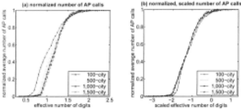
Figure 6(a) shows the average complexity of the DFBnB algorithm, measured by the number of calls to the AP func tion. The result is averaged over the same problem instances for each data point as used for the phase transitions in the pre vious section. Note that the number of AP calls increases sig nificantly from small problems to large ones using the same effective number of digits for distances. Thus, we normalize the result in such a way that for a given problem size, the min imal and maximal AP calls among all problem instances of the same size are mapped to zero and one, respectively, and the other AP calls are proportionally adjusted to a ratio between 0 and 1. This allows us to compare the results from different problem sizes on one figure. The curves in Figure 6(a) follow a pattern similar to that of the phase transitions in the previous section. The complexity of the subtour elimination algorithm increases with the effective number of digits, and exhibits a threshold behavior similar to phase transitions. Indeed, we can use finite-size scaling to capture the behavior as the problem size grows, as illustrated in Figure 6(b ). The results in Fig ure 6 and the results in the previous section indicate that the complexity of the subtour elimination algorithm goes hand-in hand with the constrainedness of the problem.
Similar results have been reported in [26]. The results of this subsection extend that in [26] to different sizes of problems and by applying finite-size scaling to capture the threshold behav ior as problem size increases.
6 Conclusions and Discussions
Our main contributions are twofold. First, we provided strong positive evidences to the long-standing question of whether the Traveling Salesman Problem (TSP) has phase transitions [17]. We studied this issue on the more general asymmetric TSP (ATSP). We empirically showed that many properties, includ ing the ATSP tour cost and the fraction of backbone, have two characteristically different values, and the transitions be tween them are rather abrupt and dramatic, displaying phase transition phenomena. The control parameter of the phase tran sitions is the effective number of digits representing the inter city distances, which in essence measures the precision of dis tances. Our results revealed the connection between distance precision and phase transition properties in the ATSP. Distance precision is the control parameter for various phase transitions of the ATSP. We believe that the concept of precision deter mining problem properties such as phase transitions is rather universal and may very well be applicable to other problems, including various scheduling and planning problems.
Second, our phase transitions results provide a practical guidance to how to generate difficult random ATSP problem instances and which instances to use to compare the asymp totic performance of two algorithms. A common practice in comparing algorithms when using a random ensemble is to generate problems with a fixed distance precision. Our results imply that the correct way is to use problem instances of dif ferent sizes that have the same or similar features such as the same fraction of backbones. This, in tum, requires to increase the number of digits for intercity distances as the problem size grows. We believe that this guidance is general and can be applied to other optimization problems.
@inproceedings{ijcai2003p171,
  title     = {Phase Transitions of the Asymmetric Traveling Salesman},
  author    = {Zhang, Weixiong},
  booktitle = {Proceedings of the Eighteenth International Joint Conference on
               Artificial Intelligence, {IJCAI-03}},
  publisher = {International Joint Conferences on Artificial Intelligence},
  editor    = {Georg Gottlob and Toby Walsh},
  pages     = {1202--1209},
  year      = {2003},
  url       = {https://ijcai.org/proceedings/2003/171},
}
TY - CPAPER TI - Phase Transitions of the Asymmetric Traveling Salesman AU - Zhang, Weixiong T2 - Proceedings of the Eighteenth International Joint Conference on Artificial Intelligence, IJCAI-03 PB - International Joint Conferences on Artificial Intelligence PY - 2003 SP - 1202 EP - 1209 UR - https://ijcai.org/proceedings/2003/171 ER -Copied
Machine-readable versions of this paper, for tools and AI agents:





