
An Improved Grid-Based Approximation Algorithm for POMDPs
Proceedings of the Seventeenth International Joint Conference on Artificial Intelligence. Pages 707-715.
© 2001 International Joint Conferences on Artificial Intelligence
Abstract
Although a partially observable Markov decision process (POMDP) provides an appealing model for problems of planning under uncertainty, exact algorithms for POMDPs are intractable. This motivates work on approximation algorithms, and grid-based approximation is a widely-used approach. We describe a novel approach to grid-based approximation that uses a variable-resolution regular grid, and show that it outperforms previous grid-based approaches to approximation.
- [Boutilier et al., 1999] Boutilier, C.; T. Dean; and S. Hanks. 1999. Decision-theoretic planning: Structural assumptions and computational leverage. Journal of Artificial Intelli- gence Research 11: 1-94.
- [Brafman, 1997] Brafman, R. 1997. A heuristic variable grid solution method for POMDPs. In Proceedings of the Fourteenth National Conference on Artificial Intelligence (AAAI-97), 727-733. Providence, RI. Cassandra et al., 1997]
- Cassandra, A.; Littman, M.; and Zhang, N. 1997. Incremental pruning: A simple, fast, exact algorithm for partially observable Markov decision processes. In Proceedings of the Thirteenth Annual Con- ference on Uncertainty in Artificial Intelligence, 54-61.
- [Drake, 1962] Drake, A. 1962. Observation of a Markov Pro- cess Through a Noisy Channel. Ph.D. thesis, Electrical En- gineering Department, M.I.T., Cambridge, MA.
- [Eckles, 1966] Eckles, J. 1966. Optimum replacement of stochastically failing systems. Ph.D. thesis, Department of Engineering-Economic Systems, Stanford University.
- [Hansen, 1998] Hansen, E. 1998. Solving POMDPs by searching in policy space. In Proceedings of the Fourteenth Conference on Uncertainty in Artificial Intelligence (UAI- 98), 211-219.
- [Hauskrecht, 1997] Hauskrecht, M. 1997. Incremental meth- ods for computing bounds in partially observable Markov decision processes. In Proceedings of the Fourteenth Na- tional Conference on Artificial Intelligence (AAAI-97), 734-739. Providence, RI.
- [Hauskrecht, 2000] Hauskrecht, M. 2000. Value-function approximations for partially observable Markov deci- sion processes. Journal of Artificial Intelligence Research 13:33-94.
- [Kakalik, 1965] Kakalik, J. 1965. Optimum policies for par- tially observable Markov systems. Technical report 18, Operations Research Center, Massachusetts Institute of Technology, Cambridge, MA.
- [Littman et al., 1995] Littman, M.; A. Cassandra; and L. Kaelbling. 1995. Learning policies for partially observable environments: Scaling up. In Proceedings of the Twelth International Conference on Machine Learning, 362-370.
- [Lovejoy, 1991] Lovejoy, W. 1991. Computationally feasible bounds for partially observed Markov decision processes. Operations Research 39:162-175.
- [Lusena et al., 1998] Lusena, C.; J. Goldsmith; and M. Mundhenk. 1998. Nonapproximability results for Markov decision processes. Technical Report, Computer Science Department, University of Kentucky.
- [Munos & Moore, 1999] Munos, R. and A. Moore. 1999. Variable resolution discretization for high accuracy solu- tions of optimal control problems. In Proceedings of 16th International Joint Conference on Artificial Intelligence. IJCAI
- [Satia & Lave, 1973] Satia, J. and Lave, R. 1973. Marko- vian Decision Processes with Probabilistic Observation of States. Management Science 20(1):1-13.
- Washington, R. 1997. BI-POMDP: Bounded, incremental partially-observable Markov-model planning. In Proceedings of the Fourth European Confer- ence on Planning (ECP-97).
- [Zhang et al., 1999] Zhang, N.; S. Lee; and W. Zhang. 1999. A method for speeding up value iteration in partially ob- servable Markov decision processes. In Proceedings of the 15th Conference on Uncertainty in Artificial Intelligence.
References were extracted automatically from the PDF and may contain errors.
Full text extracted automatically from the PDF; figures, tables and equations may differ. The PDF is the version of record.
1 Introduction
A partially observable Markov decision process (POMDP) models planning problems for which actions have stochastic effects and sensors provide imperfect and incomplete state information. Originally developed in the operations research community, this model has been adopted by the AI community as a framework for research in planning under uncertainty and related problems of reinforcement learning.
A standard approach to solving a POMDP is to transform it into an equivalent, fully observable Markov decision process with a state space that consists of all probability distributions over the core states of the POMDP, and to solve the POMDP in this form. For a POMDP with ✂ core states, the transformed state space is the ✂ -dimensional simplex, or belief simplex. Although a continuous state space such as this presents a computational challenge, discrete approximations of continuous state spaces are a natural and oftenused approximation technique. Grid-based approximation was the first approach adopted for solving POMDPs, and it is still widely-used [Drake, 1962; Kakalik, 1965; Eckles, 1966; Lovejoy, 1991; Brafman, 1997; Hauskrecht, 1997; 2000]. A finite grid is placed over the belief simplex, values are computed for points in the grid, and interpolation is used to evaluate all other points in the simplex. This is closely related to grid-approximation techniques for other continuous MDPs [Munos &Moore, 1999].
Different approaches to constructing a grid have been explored. Lovejoy (1991) describes a fixed-resolution regular grid, in which the points of the grid are spaced in a regular pattern and divide the belief simplex into equal-sized subsimplices. This allows a very efficent interpolation algorithm based on the concept of triangulation. However, the size of the grid grows exponentially with any increase in resolution. Hauskrecht (1997, 2000) and Brafman (1997) propose nonregular grids that allow the points of the grid to be spaced unevenly in the belief simplex, in order to approximate the contours of the value function as economically as possible. However, interpolation algorithms for non-regular grids are much less efficient. In this paper, we develop a variableresolution regular grid that combines the strengths of both approaches. It allows the resolution of the grid to be adjusted in different regions of the belief simplex, but in a regular pattern that makes it possible to generalize the efficient interpolation algorithm for regular grids. The result is a higher quality approximation at less computational cost.
The paper is organized as follows. We begin with a review of the POMDP model, the grid approximation approach, and Lovejoy's interpolation algorithm for regular grids. We generalize the interpolation algorithm for use with a variableresolution regular grid, and discuss methods for adjusting the resolution of the grid to achieve the best quality-time tradeoff for the approximation. We evaluate this approach analytically and experimentally, and show that it outperforms previous grid-approximation methods.
2 Background
We consider a discrete-time POMDP with a finite set of states ✄ , a finite set of actions ☎ , and a finite set of observations ✆ . Each time period, the environment is in some state ✝ ✞ ✄ , the agent takes an action ✠ ✞ ☎ for which it receives an immediate reward with expected value ☞ ✌ ✝ ✏ ✠ ✓ , the environment makes a transition to state ✝ ✕ ✞ ✄ with probability ✘ ✌ ✝ ✕ ✚ ✝ ✏ ✠ ✓ , and the agent observes ✢ ✞ ✆ with probability ✘ ✌ ✢ ✚ ✝ ✕ ✏ ✠ ✓ . Let ✦ denote a vector of state probabilities, called a belief (or information) state, where ✦ ✌ ✝ ✓ denotes the probability that the environment is in state ✝ . If action ✠ is taken and observation ✢ follows, the successor belief state, denoted ★ ✌ ✦ ✏ ✠ ✏ ✢ ✓ , is determined by revising each state probability as follows,
where ✘ ✌ ✢ ✏ ✝ ✕ ✚ ✝ ✏ ✠ ✓ ✮ ✘ ✌ ✢ ✚ ✝ ✕ ✏ ✠ ✓ ✘ ✌ ✝ ✕ ✚ ✝ ✏ ✠ ✓ and the denominator is a normalizing factor ✘ ✌ ✢ ✚ ✦ ✏ ✠ ✓ ✮ ✰ ✲ ✺ ✴ ✵ ✘ ✌ ✢ ✚ ✝ ✕ ✏ ✠ ✓ ✰ ✲ ✴ ✵ ✘ ✌ ✝ ✕ ✚ ✝ ✏ ✠ ✓ ✦ ✌ ✝ ✓ . A POMDP is solved by finding a rule for selecting actions, called a policy, that optimizes a performance objective. We assume the objective is to maximize expected total discounted reward over an infinite horizon (where ✾ ✞ ❀ ❂ ✏ ❃ ✓ is the discount factor). An optimal policy has a value function that satisfies the Bellman optimality equation,
where ☞ ✌ ✦ ✏ ✠ ✓ ✮ ✰ ✲ ✴ ✵ ✦ ✌ ✝ ✓ ☞ ✌ ✝ ✏ ✠ ✓ . Exact algorithms for solving this optimality equation are intractable for all but trivial problems. This motivates work on approximation methods.
2.1 Grid-based approximation
Let ❯ denote a grid that contains a finite set of belief states, ✦ ❱ ❲ ❳ ❳ ❳ ✦ ❱ ❪ ❱ ❪ . Abelief state ✦ is a convex combination of the belief states in grid ❯ if
where ❛ is a vector of size ✚ ❯ ✚ , ❛ ✌ ❝ ✓ ❢ ❂ for all ❛ ✌ ❝ ✓ , and ✰ ❪ ❱ ❪ ❴ ❵ ❲ ❛ ✌ ❝ ✓ ✮ ❃ . For each belief state ✦ ❱ ❴ in the grid, we store a value denoted ❦ ❧ ✌ ✦ ❱ ❴ ✓ . The convex interpolation function,
defines a continuous and piecewise-linear value function over all belief states, given values for the belief states in the grid. To compute values for the belief states in the grid, we use value iteration with the update rule,
which converges to a unique fixed-point solution that is guaranteed to be an upper bound on the optimal value function.
A belief state can be expressed as many different convex combinations of grid points. The convex combination that provides the best upper bound can be found by solving the following linear program.
Using linear programming to find the best interpolation can be very expensive. However, any convex combination provides an upper bound, and fast methods for finding a nonoptimal convex combination can produce good upper bounds. Design of a grid-approximation strategy requires addressing two questions. What interpolation method provides a good tradeoff between time and quality? What belief states should be included in the grid? Every grid must contain the corner points of the belief simplex to ensure that a convex combination can always be found. Different strategies for adding other points to a grid have been explored. We begin with a review of a fixed-resolution regular grid and the efficient interpolation algorithm it supports. In the rest of the paper, we develop a variable-resolution generalization of this.
2.2 A fixed-resolution regular grid
Lovejoy (1991) constructs a regular grid as follows. Let ✉ be a positive integer that represents the resolution of the grid. The set of belief states in the grid is defined as,
where ⑩ ❪ ✵ ❪ ❶ denotes the set of ✚ ✄ ✚ -vectors of non-negative integers. The grid divides the belief simplex into a set of equalsize sub-simplices. Note that when ✉ ✮ ❃ , the grid contains only the corner points of the simplex. The number of points in the grid is given by the formula:
The advantage of a regular grid is that it allows an elegant and efficient method of interpolation. To evaluate a belief state ✦ requires finding the vertices of the smallest subsimplex that contains ✦ , and then finding the coefficients of interpolation ❛ ✌ ❝ ✓ . Lovejoy defines a second grid of integer vectors,
and converts a belief state ✦ ✞ ❯ into an integer vector ➉ ✞ ❯ ✕ in order to perform interpolation. Because of a one-to-one correspondence between grid points in ❯ and ❯ ✕ , the subsimplex that contains ➉ ✞ ❯ ✕ can be used to determine the sub-simplex that contains ✦ ✞ ❯ . Here, we summarize the steps of the interpolation algorithm. We refer to Lovejoy (1991) for a detailed explanation.
- Given a belief state ➌ , create an ➍ ➎ ➍ -vector ➏ such that ➏ ➐ ➑ ➒ ➓ ➔ ✰ → ➣ → ↔ ↕ ➙ ➌ ➐ ➝ ➒ for ➞ ➟ ➑ ➟ ➍ ➎ ➍ . (This transforms probability density function ➌ into cumulative distribution function ➏ .)
- Let ➠ be the largest integer ➍ ➎ ➍ -vector such that ➠ ➐ ➑ ➒ ➟ ➏ ➐ ➑ ➒ for all ➑ ➢ ➎ .
- Let ➥ be an ➍ ➎ ➍ -vector such that ➥ ➐ ➑ ➒ ➓ ➏ ➐ ➑ ➒ ➧ ➠ ➐ ➑ ➒ for all ➑ ➢ ➎ .
- Let ➫ be an ➍ ➎ ➍ -vector that contains a permutation of the integers ➞ ➭ ➯ ➭ ➳ ➳ ➳ ➭ ➍ ➎ ➍ that orders the components of ➥ in descending fashion, so that ➥ ➐ ➫ ➐ ➞ ➒ ➒ ➺ ➥ ➐ ➫ ➐ ➯ ➒ ➒ ➺ ➳ ➳ ➳ ➺ ➥ ➐ ➫ ➐ ➍ ➎ ➍ ➒ ➒ .
- Find the vertices ➻ ➠ ↔ ➽ ➞ ➟ ➝ ➟ ➍ ➎ ➍ ➶ of the sub-simplex in ➹ ➘ that contains ➏ , as follows:
By the isomorphism between ➹ and ➹ ➘ , this identifies the corresponding vertices ➻ ➌ ❒ ↔ ➽ ➞ ➟ ➝ ➟ ➍ ➎ ➍ ➶ of the sub-simplex in ➹ that contains ➌ .
- Find the barycentric coordinates ➻ ❰ ➐ ➝ ➒ ➽ ➞ ➟ ➝ ➟ ➍ ➎ ➍ ➶ for the interpolation, as follows:
The complexity of each of these steps is a212 ✌ ✚ ✄ ✚ ✓ , with the possible exception of step 4 which requires sorting the elements of an ✚ ✄ ✚ -vector. Although sorting has worst-case complexity a212 ✌ ✚ ✄ ✚ a214 a215 ✚ ✄ ✚ ✓ , we can improve this by noting that the difference vector a216 is uniformly distributed over ❀ ❂ ✏ ❃ ✓ . Bucket sort is ideally suited for input data that is uniformly distributed between 0 and 1, and has only linear average-case complexity. Using bucket sort, the average-case complexity of the interpolation algorithm is a212 ✌ ✚ ✄ ✚ ✓ . We note the important fact that the complexity of interpolation does not depend on the size of the grid.
We store the grid using a hash table. Our hash function uses lexicographical ordering of the integer vectors in ❯ ✕ to map each vector in ❯ ✕ to a unique integer from ❂ to ✌ ✉ ■ ✚ ✄ ✚ ❽ ❃ ✓ ❾ a219 ✉ ❾ ✌ ✚ ✄ ✚ ❽ ❃ ✓ ❾ ✓ ❽ ❃ . The hash function is perfect if the size of the hash table is equal to or greater than ✌ ✉ ■ ✚ ✄ ✚ ❽ ❃ ✓ ❾ a219 ✉ ❾ ✌ ✚ ✄ ✚ ❽ ❃ ✓ ❾ ✓ , which is the total number of possible grid points. (The hash function assumes a maximum resolution, ✉ .) Because the number ✌ ✉ ■ ✚ ✄ ✚ ❽ ❃ ✓ ❾ a219 ✉ ❾ ✌ ✚ ✄ ✚ ❽ ❃ ✓ ❾ ✓ ❽ ❃ explodes quickly as ✉ and ✚ ✄ ✚ increase, it is usually impossible to have a hash table this large. We resolve collisions by associating a linked list with each slot, and use the hash code to uniquely identify the grid point in the list.
3 A variable-resolution regular grid
The disadvantage of a fixed-resolution grid is that increasing the resolution of the value function approximation in one region of the belief simplex requires increasing its resolution everywhere. This causes an exponential explosion in the size of the grid, and makes this approach infeasible for all but small problems. To address this problem, Lovejoy (1991) suggested a variable-resolution generalization of his method that would "maintain the simplicity of the Freudenthal triangulation, but allow the mesh ✉ to vary on different portions of a222 ✌ ✄ ✓ ." However, neither Lovejoy nor anyone else developed this extension.
In the rest of this paper, we develop this variable-resolution generalization of Lovejoy's regular grid. We discuss how to generalize the Freudenthal interpolation and how to select the appropriate resolution for different regions of the simplex. In allowing the resolution of the grid to vary, we adopt the rule that the resolution ✉ is always a positive integer power of 2. This ensures that vertices of low-resolution sub-simplices are also vertices of higher-resolution sub-simplices, and still useful when resolution is increased. From now on, we let ✉ denote the highest resolution anywhere in the grid.
3.1 Interpolation
Smallest complete sub-simplex To perform interpolation for belief state ✦ , we search for the smallest (i.e., highestresolution) sub-simplex containing ✦ that is complete (i.e., all its vertices are in the grid). The lowest possible resolution of the grid is 1, and the highest possible resolution, ✉ , is given. (We must know ✉ in order to create the hash function for the hash table used to store the grid.) For any resolution, the algorithm summarized in Section 2.2 identifies the vertices of the sub-simplex containing ✦ , and we can check whether all of these are in the grid. Thus, we can use binary search to find the resolution between 1 and ✉ with the smallest complete sub-simplex containing ✦ . Because the grid always includes the corner points of the belief simplex, the search is guaranteed to find a complete sub-simplex at some resolution. The complexity of this interpolation algorithm is a212 ✌ ✚ ✄ ✚ a214 a215 a214 a215 ✉ ✓ , where the factor a214 a215 a214 a215 ✉ reflects the complexity of binary search and the fact that only resolutions that are powers of two must be considered.
Virtual points Each point in a regular grid is a vertex in many different sub-simplices. In a variable-resolution grid in which not every part of the grid is refined to the same resolution, this means that there will be many sub-simplices for which some but not all of their vertices are grid points. The smallest complete algorithm considers sub-simplices containing ✦ at different resolutions, until it finds the smallest complete one. In its search, it always considers the sub-simplex at the next higher resolution. Even though this sub-simplex is not complete, many of its vertices may be present in the grid. It can be advantageous to use these higher-resolution grid points in interpolation, and it is possible to do so by "filling in" the missing vertices with what we call virtual vertices. Any vertex that is missing from a sub-simplex is a belief state for which we can create an upper bound value by performing interpolation, since the missing vertex is contained in a lowerresolution sub-simplex. We call this computed value a virtual vertex. By using virtual vertices to fill in the missing vertices of the incomplete sub-simplex at the next higher resolution after the smallest complete one, we can improve the interpolated value. The cost for this improvement is an increase in the worst-case complexity of interpolation by a factor of ✚ ✄ ✚ compared to the smallest complete algorithm (since in the worst case every vertex may be missing from a sub-simplex). But this complexity factor can be improved by not creating virtual vertices for an incomplete sub-simplex with more than MaxVirtual vertices missing. This limits the increase in worst-case complexity to a factor of MaxVirtual ♣ ✚ ✄ ✚ . In practice, we found that another technique significantly reduces the average-case complexity of virtual interpolation without adversely affecting the result. For an incomplete subsimplex, let ❛ Sum denote the sum of the barycentric coordinates for vertices that are present. (Note that ❛ sum ✞ ❀ ❂ ✏ ❃ ✓ for an incomplete sub-simplex.) We don't perform virtual interpolation for a sub-simplex for which ❛ Sum a224 ❛ Threshold. Adjusting this threshold lets us adjust a time-quality tradeoff for this method of interpolation. We report experimental results for different threshold values in Section 4.
3.2 Refining the grid
We now discuss the question of how to refine the grid, that is, how to selectively adjust the resolution of the grid in different regions of the belief simplex. A natural strategy is to do so in a way that reduces the error of the approximation. This requires a method for estimating the error. Since our gridbased approximation is an upper bound on the optimal value function, the error can be estimated by measuring its distance from a lower-bound function.
Lovejoy (1991) discusses how to use a grid to compute a lower-bound function, as well as an upper-bound function. The lower-bound function is represented by a set of ✚ ✄ ✚ -vectors, a225 ✮ a227 a229 ❲ ✏ a229 ➄ ✏ ❳ ❳ ❳ ✏ a229 ❪ ❱ ❪ a230 , with the value of belief state ✦ computed as follows,
One vector is associated with each grid belief state, and is computed by value iteration using the following update rule.
- For each action a236 and observation a237 , let
- For each action a236 , let
The complexity of performing this update for every grid belief state is a212 ✌ ✚ ❯ ✚ ✚ ☎ ✚ ✚ ✆ ✚ ✚ ✄ ✚ ➄ ✓ . Although value iteration using this update is guaranteed to produce a value function that is a lower bound on the optimal value function, it may not converge to a fixed point. Hauskrecht (1997, 2000) and Zhang et al. (1999) propose refinements of this update that guarantee convergence, but they fail to bound the size of a225 or the complexity of the update. So we do not use their refinements.
Given these upper and lower-bound grid-based value functions, Lovejoy describes an algorithm that computes a uniform error bound (which is the maximum difference between the upper and lower-bound functions for any belief state). Unfortunately, it has complexity a212 ✌ ✚ ✄ ✚ ❾ ✚ ❯ ✚ ➄ ✓ , and our experience indicates that it is intractable for problems with more than nine or ten states. However, Lovejoy notes that it is easy to compute an approximate error bound (defined as the maximum difference between the upper and lower-bound functions for any grid belief state). This is guaranteed to be tighter than the uniform bound, and we can use it to refine the grid.
Once we have identified the grid point(s) with the largest error, what belief states should we add to the grid in order to reduce the error at these points? The value of a grid belief state depends on the interpolated value of its successor belief states, so refining the grid at the successor belief states will reduce the error at the grid point. For a successor belief state ✦ , we increase the resolution of the grid by adding the vertices of the ✆ ✉ -resolution sub-simplex containing ✦ to the grid, where ✉ is the resolution of the smallest complete subsimplex containing ✦ in the current grid. This adds at most ✚ ✄ ✚
points to the grid, which is the maximum number of missing vertices in the higher-resolution sub-simplex.
This first approach to refining the grid tries to improve the grid-based approximation everywhere, without considering reachability from a start state. If the starting belief state for a POMDP is given, a policy can be found using forward search [Satia & Lave, 1973; Washington, 1997; Hansen, 1998; Hauskrecht, 2000]. This focuses computation on regions of the belief simplex that are reachable from the starting belief state. Upper and lower-bound functions can be used to prune branches of the search tree, as well as to compute an error bound for the starting belief state (by backing-up upper and lower-bound values from the leaves of the search tree to the root). This suggests a more focused approach to refining grid-based upper and lower-bound functions: attempt to reduce the error bound of the belief state at the root of the search tree. This can be done by refining the grid for belief states on the fringe of the search tree that contribute most to the value of the starting belief state.
Although we choose to focus on grid-refinement strategies that attempt to reduce the error bound of the approximation, other strategies are possible. For example, given upper and lower-bound value functions, it is sometimes possible to identify the optimal action for a belief state using action elimination. It may be desirable to refine the grid at points where the optimal action is uncertain, and by the same reasoning, unnecessary to refine it at points where the optimal action can be determined, regardless of the error bound at these points. Hauskrecht (1997, 2000) and Brafman (1997) suggest other heuristics for choosing points to add to a (non-regular) grid. These heuristics consider such factors as reachability, likely improvement of corner points of belief simplex, and likely effect on the policy, and can be viewed as complementary to our strategy of reducing an error bound.
3.3 Comparison to non-regular grids
A variable-resolution regular grid is not the only way to allow the resolution of a grid to vary in different regions of the belief simplex. Another approach is a non-regular grid that allows the points of the grid to occur anywhere in the belief simplex, and not necessarily in a regular pattern that allows for triangulation. Hauskrecht (1997, 2000) and Brafman (1997) propose non-regular grids, and we now compare this approach to our variable-resolution regular grid.
A drawback of non-regular grids is that interpolation is more difficult. Hauskrecht proposes an interpolation algorithm that creates a convex combination using one point in the grid and ✚ ✄ ✚ ❽ ❃ corner points of the belief simplex. Because it tests each point in the grid in order to select the one that gives the best interpolated value, its complexity is a212 ✌ ✚ ❯ ✚ ✚ ✄ ✚ ✓ . Brafman proposes an interpolation algorithm that relies on the grid belief states being sorted in decreasing order of entropy. Given a belief state ✦ for which interpolation is to be performed, Brafman's algorithm searches the list of grid belief states until a belief state ✦ ❱ ❴ is found that assigns positive probability only to states to which ✦ assigns positive probability. The maximum coefficient ✝ for which ✌ ✦ ❽ ✝ ✟ ✦ ❱ ❴ ❢ ❂ ✓ is calculated, and the process is repeated with ✌ ✦ ❽ ✝ ✟ ✦ ❱ ❴ ✓ instead of ✦ until interpolation is complete. (Searching a list sorted by entropy has the effect of prefering low-information belief ☞ states that are likely to be closer to ✦ .) The algorithm has worst-case complexity a212 ✌ ✚ ❯ ✚ ✚ ✄ ✚ ➄ ✓ , and requires an initial sort with complexity a212 ✌ ✚ ❯ ✚ a214 a215 ✚ ❯ ✚ ✚ ✄ ✚ ✓ . Although both interpolation algorithms are simple, their complexity depends on the size of the grid. This is a serious drawback that limits the size of non-regular grids in practice.
3.4 Value iteration
Although the complexity of interpolation in regular grids does not depend on the size of the grid, the complexity of value iteration in both regular and non-regular grids does. Values for grid belief states are computed using value iteration, with values initialized to known upper bounds (such as their completely observable values). In a variable-resolution regular grid, the compexity of the first iteration of value iteration is a212 ✌ ✚ ❯ ✚ ✚ ☎ ✚ ✚ ✆ ✚ ✚ ✄ ✚ ➄ a214 a215 a214 a215 ✉ ✓ , where ✚ ❯ ✚ is the number of grid points, ✚ ☎ ✚ ✚ ✆ ✚ is the number of successor belief states of each grid point, ✚ ✄ ✚ ➄ is the worst-case complexity of computing a successor belief state by Bayesian conditioning, and a214 a215 a214 a215 ✉ reflects the added complexity of interpolation. Because both successor belief states and barycentric coordinates used for interpolation can be cached for re-use, the complexity of subsequent iterations of value iteration is only a212 ✌ ✚ ❯ ✚ ✚ ☎ ✚ ✚ ✆ ✚ ✚ ✄ ✚ ✓ , where ✚ ✄ ✚ is the complexity of computing an interpolated value using the cached barycentric coordinates. In practice, caching successor belief states and barycentric coordinates dramatically improves the running time of value iteration.
Because the same successor belief states and barycentric coordinates are used in each iteration of value iteration, this grid-based approximation is a finite-state MDP and convergence to a fixed-point solution in polynomial time is guaranteed [Hauskrecht, 2000]. In non-regular grids, the barycentric coordinates used for interpolation are re-computed each iteration. Because the complexity of interpolation in nonregular grids depends on ✚ ❯ ✚ , the complexity of each iteration of value iteration in a non-regular grid is quadratic in ✚ ❯ ✚ . This underscores the advantage of using a regular grid.
In addition to limiting the complexity of interpolation, it is helpful to limit the factor ✚ ❯ ✚ ✚ ☎ ✚ ✚ ✆ ✚ , which is the number of times interpolation (and other calculations involved in computing a backup) are performed in each iteration of value iteration. The obvious way to limit this factor is to limit the size of the grid. This adjusts a tradeoff between quality of approximation and grid size, and a variable-resolution grid lets us space the points of the grid to achieve the best possible approximation for a given grid size. Action eliminations can be used to limit ✚ ☎ ✚ . As for ✚ ✆ ✚ , it may be reduced by ignoring some, or all, observations, and evaluating the successor belief states of actions. If grid-based interpolation is used to evaluate the successor belief states of actions, however, the gridbased approximation may no longer be an upper bound. The upper bound guarantee is lost because information provided by the observation is ignored. (The upper bound guarantee can be restored by using the corner points of the belief simplex to perform interpolation, since this is equivalent to assuming perfect information, but this impairs the quality of the approximation. If always done, the grid-based approximation becomes no better than the completely observed heuristic.)
Finally, we note that it is possible to improve a grid-based approximation without adding points to the grid. Instead of performing a conventional backup using one-step lookahead, the value of a grid point can be improved further by using a deeper lookahead search that we call a multi-step backup. Using branch-and-bound or AO* search, the upper-bound function can be used to prune the search tree and the depth of the lookahead can adjust a tradeoff between search complexity and improvement of of value. We report some experimental results for this technique in the next section.
4 Performance Results
We experimentally evaluate our grid-based approximation algorithm using several test problems from the literature. These include the machine maintenance problem that is Lovejoy's (1991) only test example; the four most-difficult-to-solve problems from a test set used by Cassandra et al. (1997) (see Table 1); the 20-state, 6-action, 8-observation gridworld navigation problem used as a test example by Hauskrecht (1997, 2000); and the 89-state, 5-action, 17-observation gridworld navigation problem introduced by Littman et al. (1995) and used as a test example by Brafman (1997).
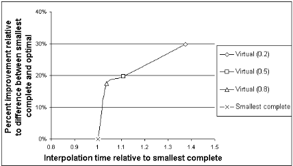
Interpolation We first compare the time-quality tradeoff for different methods of interpolation in a variable-resolution regular grid. We use the five small test problems in Table 1 for this comparison, so that we can also compute an optimal interpolation using linear programming. Figure 1 shows the performance of interpolation using virtual points relative to performance using the smallest complete subsimplex method alone. We measure improvement as a percentage of the difference between the interpolated value using the smallest complete method and the optimal interpolated value. Virtual point interpolation is tested with three different ❛ Sum threshold values; 0.2, 0.5, and 0.8. As expected, a smaller ❛ Sum threshold achieves better quality at the cost of speed. For these problems, virtual point interpolation takes only slightly longer than the smallest complete sub-simplex method. (Interpolation using linear programming runs an average of 16 times slower.) For problems with larger state spaces, virtual point interpolation takes relatively longer because its worst-case complexity is quadratic in the size of the state space instead of linear, but reasonable performance can still be achieved by adjusting the ❛ Sum threshold. Optimal interpolation using linear programming is infeasible for larger problems.
| Fixed resolution | Variable resolution | |||||||||||
|---|---|---|---|---|---|---|---|---|---|---|---|---|
| Problem | ➍ ➎ ➍ | ➍ ✌ ➍ | ➍ ✍ ➍ | Error | M | ➍ ➹ ➍ | UB time | LB time | M | ➍ ➹ ➍ | UB time | LB time |
| Machine Maintenance | 3 | 4 | 2 | 0.02 | 20 | 231 | 0.5 | 63.2 | 64 | 45 | 3.04 | 7.98 |
| Network Monitoring | 7 | 4 | 2 | 36.41 | 4 | 210 | 1.44 | 84.69 | 8 | 71 | 7.07 | 7.57 |
| Shuttle Docking | 8 | 3 | 5 | 0.38 | 4 | 330 | 0.43 | 128.29 | 8 | 47 | 0.35 | 4.08 |
| Navigation | 12 | 4 | 6 | 0.03 | 4 | 1365 | 3.74 | 2133.3 | 32 | 299 | 5.34 | 149.86 |
| Aircraft Identification | 12 | 6 | 5 | 0.29 | 4 | 1365 | 7.62 | 4378.4 | 8 | 186 | 2.57 | 80.43 |
Interpolated values are typically close to optimal. There appear to be two reasons for sub-optimality. First, interpolation using a sub-simplex is less flexible than interpolation using a convex combination. (Every sub-simplex is a convex combination, but not every convex combination is a subsimplex.) As a result, better interpolated values can sometimes be found using convex combinations that do not correspond to sub-simplices. The second reason is more problematic. Although the interpolation function is piecewise linear and continuous, there is no guarantee that it is convex. For most problems, we found that it is convex (or nearly so). However, we sometimes found non-convexities. When they exist, the "nearest" grid points do not necessarily give the best interpolation. We found non-convexities in two of our test problems: the networkmonitoring problem fromCassandra's test set and Hauskrecht 20-state grid navigation problem. The large error bound for the network monitoring problem in Table 1 reflects this. Note that these non-convexities occur in both fixed-resolution and variable-resolution regular grids.
One explanation for non-convexity is that "localized" transitions may prevent values from propagating throughout the grid. That is, non-convexities may occur when improved values in one area of the grid do not improve values in another area of the grid because there is not a chain of successor belief states between them through which they can propagate.
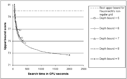
For both test problems with non-convexities, we found that multi-step backups corrected the problem. (Multi-step backups are described in the last paragraph of Section 3.4.) Instead of refining the grid at points with the largest error bound, we performed multi-step backups at these points. For the network monitoring problem, using multi-step backups with a depth bound of ten reduced the error bound from 36.41 to 0.7 after 150 CPU seconds. Figure 2 shows the positive effect of multi-step backups on Hauskrecht's 20-state maze problem. (For this problem, the upper bound score is defined as the average value of a fixed set of 1000 randomly generated belief states plus the corner points, a metric Hauskrecht uses.) For the other test problems, multistep backups do not improve the value function as much as grid refinement does. As a rule of thumb, when the error bound for a problem remains large despite grid refinement, multi-step backups may correct the problem.
Refining the grid Table 1 compares the performance of a fixed-resolution grid and a variable-resolution grid on five small test problems. Each problem is solved using a fixedresolution regular grid, and the error bound is measured. Then a variable-resolution grid is used to find a solution with the same error bound. We use virtual interpolationwith ❛ Sum = 0.5, for the variable-resolution grid. The results show that a variable-resolution approximation can achieve the same accuracy with a much smaller grid.
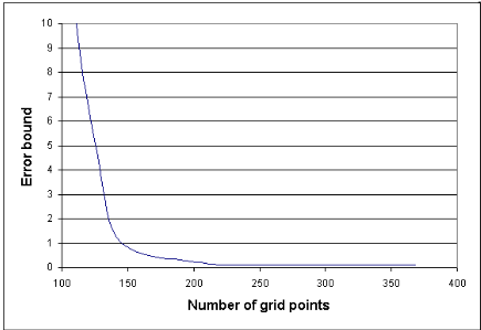
Figure 3 shows how the error bound decreases as the size of grid increases for the Aircraft Identification problem. Results are similar for other problems. Using the error bound to determine where to refine the grid requires a lower bound function, but Lovejoy's grid-based lower bound function can be time-consuming to compute. For the 89-state hallway navigation problem, computing an ✚ ✄ ✚ -vector for each and every grid point is prohibitive. But it is not necessary. In our experiments with the hallway problem, we got good results using a lower-bound function consisting of only ten ✚ ✄ ✚ -vectors. Each iteration, we computed an ✚ ✄ ✚ -vector for the ten grid points with the largest error bound.
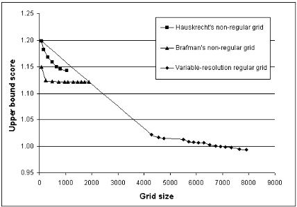
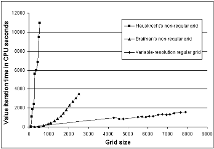
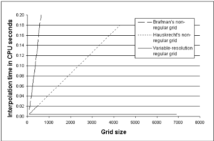
Comparison to non-regular grids Figure 4 shows how the quality of the upper bound function improves as the size of the grid increases for the 89-state hallway navigation problem. It also shows that a better upper bound function can be computed using a variable-resolution regular grid than using a non-regular grid. The reason for this is that faster interpolation makes it possible to use a much larger grid. Figure 5 shows average interpolation time as a function of grid size for our regular grid, compared to Brafman's and Hauskrecht's non-regular grids, and dramatically underscores the advantage of regular grids. Figure 6 compares the time it takes value iteration to converge for each of these methods, as a function of grid size. Although the variable-resolution regular grid is much larger, it takes less time to compute. Brafman's value iteration algorithm is faster than Hauskrecht's (even though his interpolation algorithm is slower), because it disregards observations and only considers the successor belief states of actions. Even with this simplification, value iteration in Brafman's non-regular grid is slower than value iteration in a regular grid. Moreover, as noted earlier, ignoring observations means that his grid-based approximation is not guaranteed to be an upper bound (although the values it computes for this problem are, in fact, upper bounds).
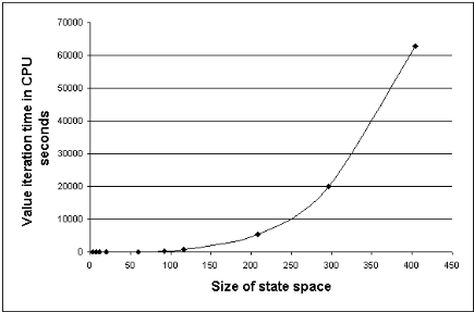
Figure 7: Increase in value iteration time in a fixed-resolution regular grid with M = 2, as a function of state space size.
Scalability Although a variable-resolution regular grid allows much larger grids (and thus better approximations), the size of the state space remains a problem in scaling-up this approach. Figure 7 compares the time it takes to compute a regular grid for a succession of POMDP problems with increasing state space size. (All problems have 5 actions and 17 observations.) Besides confirming that the size of the state space is the primary factor that limits the scalability of grid-based approximation, this gives some idea of the range of problems for which grid-based approximation is currently feasible. We have found that almost all of the running time of value iteration is spent performing interpolation or computing successor ✎ belief states using Bayesian conditioning, and the complexity of both depends on the size of the state space. This points to where further work on grid-based approximation is needed. In order to improve the efficiency of interpolation and Bayesian conditioning for problems with larger state spaces, we need to integrate grid-based approximation with various techniques for state abstraction that have been explored for MDPs and POMDPs [Boutilier et al., 1999]. (State abstraction would also make it possible to compute Lovejoy's grid-based lower-bound function more efficiently.)
5 Discussion
POMDPs are notoriously difficult to solve, and finding even a bounded-optimal solution is an intractable problem [Lusena et al., 1998]. Grid-based approximation algorithms have polynomial-time complexity in the size of the grid and the number of states, actions, and observations [Hauskrecht, 2000]. Although there is no guarantee on the quality of the approximation that can be achieved in polynomial time, a well-designed grid-based approximation can be adjusted in several ways to optimize a time-quality tradeoff.
This paper introduces a variable-resolution regular grid that allows the resolution of the grid to be adjusted in different regions of the belief simplex, in order to approximate the contours of the value function as efficiently as possible. Although non-regular grids also allow this, interpolation in nonregular grids is more difficult and its complexity is a function of the size of the grid. In a variable-resolution regular grid, the complexity of interpolation is independent of the size of the grid. Thus, it is feasible to use much larger grids with this approach in order to achieve better approximations.
Our experiments indicate that it is easier to scale up this approach to large grids than to large state spaces, and the size of the state space remains the most prohibitive factor in the complexity of grid-based approximation. To use grid-based approximation to solve POMDPs with large state spaces, we need to integrate it with various techniques for state abstraction that have been explored for MDPs and POMDPs. This is a promising direction for future research.
Acknowledgments
We thank Tony Cassandra and Milos Hauskrecht for making available their test problems, and the anonymous reviewers for helpful comments. This research is supported in part by the National Science Foundation under grant IIS-9984952.
@inproceedings{ijcai2001p97,
  title     = {An Improved Grid-Based Approximation Algorithm for POMDPs},
  author    = {Zhou, Rong and Hansen, Eric A.},
  booktitle = {Proceedings of the Seventeenth International Joint Conference on
               Artificial Intelligence, {IJCAI-01}},
  publisher = {International Joint Conferences on Artificial Intelligence},
  editor    = {Bernhard Nebel},
  pages     = {707--715},
  year      = {2001},
  url       = {https://ijcai.org/proceedings/2001/97},
}
TY - CPAPER TI - An Improved Grid-Based Approximation Algorithm for POMDPs AU - Zhou, Rong AU - Hansen, Eric A. T2 - Proceedings of the Seventeenth International Joint Conference on Artificial Intelligence, IJCAI-01 PB - International Joint Conferences on Artificial Intelligence PY - 2001 SP - 707 EP - 715 UR - https://ijcai.org/proceedings/2001/97 ER -Copied
Machine-readable versions of this paper, for tools and AI agents:





