
Splitting Without Backtracking
Proceedings of the Seventeenth International Joint Conference on Artificial Intelligence. Pages 611-616.
© 2001 International Joint Conferences on Artificial Intelligence
Abstract
Integrating the splitting rule into a saturation-based theorem prover may be highly beneficial for solving certain classes of first-order problems. The use of splitting in the context of saturation-based theorem proving based on explicit case analysis (as implemented in SPASS) employs backtracking which is difficult to implement as it affects design of the whole system. Here we present a “cheap” and efficient technique for implementing splitting that does not use backtracking.
- [Bachmair and Ganzinger, 2001] L. Bachmair and H. Ganzinger. Resolution theorem proving. In A. Robinson and A. Voronkov, editors, Handbook of Automated Reasoning, volume I, chapter 2, pages 19-99. Elsevier Science, 2001.
- [Fermüller et al., 2001] C. Fermüller, A. Leitsch, U. Hustadt, and T. Tammet. Resolution decision procedures. In A. Robinson and A. Voronkov, editors, Handbook of Automated Reasoning, volume II, chapter 25, pages 1791-1849. Elsevier Science, 2001.
- [Joyner, Jr., 1976] William H. Joyner, Jr. Resolution strategies as decision procedures. Journal of the ACM, 23(3):398-417, July 1976.
- [Riazanov and Voronkov, 2000a] A. Riazanov and A. Voronkov. Limited resource strategy in resolution theorem proving. Preprint CSPP-7, Department of Computer Science, University of Manch- ester, October 2000.
- [Riazanov and Voronkov, 2000b] A. Riazanov and A. Voronkov. Partially adaptive code trees. In M. Ojeda-Aciego, I.P. de Guzmán, G. Brewka, and L.M. Pereira, editors, Logics in Artificial Intelligence. European Workshop, JELIA 2000, volume 1919 of Lecture Notes in Artificial Intelligence, pages 209-223, Málaga, Spain, 2000. Springer Verlag.
- [Riazanov and Voronkov, 2001] A. Riazanov and A. Voronkov. Vampire 1.1 (system description). Siena, Italy, June 2001. Ac- cepted to IJCAR 2001.
- [Schumann and Fischer, 1997] J. Schumann and B. Fischer. NORA/HAMMR: Making deduction-based software component retrieval practical. In Proc. Automated Software Engineering (ASE-97), pages 246-254, Lake Tahoe, November 1997. IEEE Computer Society Press.
- [Sutcliffe and Suttner, 1998] G. Sutcliffe and C. Suttner. The TPTP problem library -CNF release v. 1.2.1. Journal of Automated Reasoning, 21(2), 1998.
- [Voronkov, 1995] A. Voronkov. The anatomy of Vampire: Imple- menting bottom-up procedures with code trees. Journal of Auto- mated Reasoning, 15(2):237-265, 1995.
- [Weidenbach et al., 1999] C. Weidenbach, B. Afshordel, U. Brahm, C. Cohrs, T. Engel, E. Keen, C. Theobalt, and D. Topic. System description: SPASS version 1.0.0. In H. Ganzinger, editor, Auto- mated Deduction-CADE-16. 16th International Conference on Automated Deduction, volume 1632 of Lecture Notes in Artificial Intelligence, pages 378-382, Trento, Italy, July 1999.
References were extracted automatically from the PDF and may contain errors.
Full text extracted automatically from the PDF; figures, tables and equations may differ. The PDF is the version of record.
1 Introduction
Case analysis in the form of the ✁ -rule is the core of tableaubased theorem proving methods. If our aim is to refute a set of clauses ✂ ✄ ✆ ✞ ✠ ☛ ✌ , we can reduce this task to refuting two simpler sets: ✂ ✄ ✆ ✞ ✌ and ✂ ✄ ✆ ☛ ✌ . This is justified by the following argument. To show that ✂ is false in all the models of the formula ✞ ✠ ☛ , one can separately consider two cases: all the models of ✞ and the ones not necessarily satisfying ✞ but satisfying ☛ . The saturation based theorem proving has adopted the case analysis principle in the form of splitting that can be formulated in the propositional case as the following inference rule:
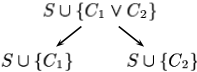
where ✂ is a set of clauses, ✪ ✫ and ✪ ✭ are clauses. Unlike most of the other inference rules in saturation-based theorem proving that only modify a set of clauses by adding and removing some clauses, this rule makes two sets of clauses out of one. Now, to refute the original set ✂ ✄ ✆ ✪ ✫ ✠ ✪ ✭ ✌ , one must separately refute the two new sets: ✂ ✄ ✆ ✪ ✫ ✌ and ✂ ✄ ✆ ✪ ✭ ✌ .
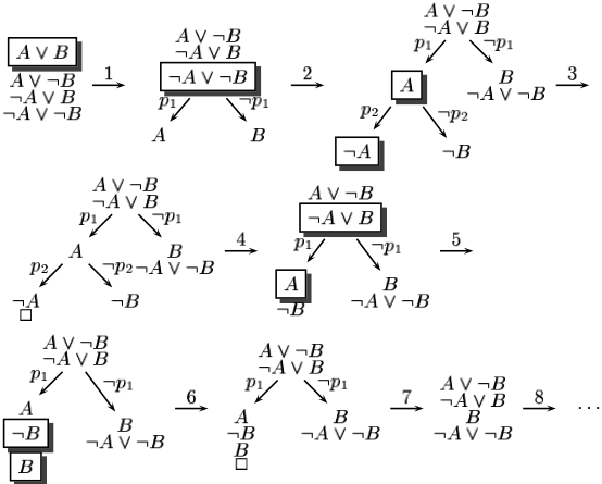
In the propositional case, this rule together with unit resolution gives a complete inference system. Finding a refutation in this system can be organised, for example, as depth-first exploring of branches. After finding a refutation on one of the splitting branches, the procedure backtracks and proceeds with the second branch. In what follows, we call this procedure explicit case analysis. A simple example of a propositional derivation which combines the splitting rule with resolution on branches is shown in Figure 1. The current search state is depicted as a tree. The nodes contain clauses common for all the branches below them. The clause or clauses to which an inference rule has been applied is put in a shaded box. For a moment, ignore the labels of the edges, for example ✶ ✫ .
✵ Partially supported by grants from EPSRC and the Faculty of Science and Technology, the University of Manchester. The first author is also partially supported by an ORS award.
In the first-order case the splitting rule can be formulated in the same way as in the propositional case with an additional restriction: the clauses ✪ ✫ and ✪ ✭ do not have common variables. This rule can be combined with inference rules like resolution and paramodulation. Combined with some resolution strategies, it gives decision procedures for fragments of first-order logic (see e.g. [Ferm¨ uller et al., 2001]).
The cost of naive backtracking is very high, since the clause set ✂ can contain tens of thousands of clauses, so after several splits a lot of memory is needed to store backtrack points. Therefore, in practice (the SPASS prover [Weidenbach et al., 1999]) explicit case analysis is implemented by adding to each clause its split history: the set of splits used to obtain this clause, represented by an array of bits. The split history also helps to implement intelligent backtracking: by analyzing the split history one can check which splits have actually been used to obtain a contradiction on the current branch.Clauses which do not belong to the currently exploited branch are put in a special waiting list, and popped back from the waiting list upon backtracking. There are complications caused by simplification by unit equalities belonging to a branch which can be illustrated by the following example.
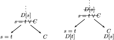
Example 1.1 Consider the split on the left of this picture:
. . .
where ✪ and ❁ ❂ ❃ have no common variables, ❁ ❅ ❃ in the simplification order used in the proof-search, and ❇ ❈ ❁ ❊ is a clause with an occurrence of ❁ . After the split the left branch contains two clauses ❁ ❂ ❃ and ❇ ❈ ❁ ❊ , so ❇ ❈ ❁ ❊ can be simplified and replaced by ❇ ❈ ❃ ❊ , but only on the left branch, since there is no clause ❁ ❂ ❃ on the right branch. This means that ❇ ❈ ❁ ❊ should still be kept on the right branch, so simplification by ❁ ❂ ❃ should be implemented according to the right-hand side of the picture.
To achieve efficiency, modern theorem provers maintain one or more indexes on terms, literals, or clauses. To implement splitting, maintainance and retrieval algorithms on indexes should be changed. Either one should have common indexes for all branches, or else indexes for the current branch only. In the former case, index retrieval algorithms should be changed to take into attention the splitting history. In the latter case, index maintainance algorithms should be changed. In either case, a significant amount of work on indexes is required upon backtracking.
In general, backtracking in resolution-based theorem provers requires a nontrivial implementation. In the modern saturation-based theorem provers for first-order logic, splitting with backtracking is implemented only in SPASS [Weidenbach et al., 1999].
In this report we discuss an alternative to the explicit case analysis which can be implemented in resolution-based theorem provers without a significant overhead. We call it splitting without backtracking. The idea of splitting without backtracking can be formulated as follows. Consider again the split of Example 1.1, but let us mark the branches of the search tree by literals as follows. We take a new propositional symbol ✶ and mark the left branch with ✶ and the right branch with ❭ ✶ :
. . .
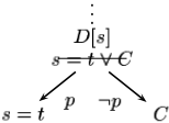
If there are several splits, we introduce a new propositional symbol for every split. Now, instead of dealing with branches, we simply add to each clause on a branch all labels used on that branch. Then the split can be described as the following inference rule which replaces a clause by two new clauses:
It is not hard to argue that such a splitting preserves the unsatisfiability of the set of clauses (we will prove it formally below). The effect of splitting is very similar to the effect of the explicit case analysis, but branches are no more needed, since we are still dealing with just one set of clauses. The following simplification of ❇ ❈ ❁ ❊ by ❁ ❂ ❃ on the left branch can now be described in at least two possible ways:
The second way corresponds to the simplification of Example 1.1, but we prefer the first way because it gives simpler clauses.
We will show that splitting without backtracking can simulate, in some sense, explicit case analysis. Moreover, by using various selection functions one can simulate a parallel version of case analysis, in which branches are exploited simultaneously. Apart from being easy to implement, splitting without backtracking has several other advantages: firstly, we obtain the effect of intelligent backtracking for free, and secondly ♦ , some simplification rules can move clauses between the branches thus avoiding repeated work on different branches.
This article is organized as follows. In Section 2 we define some fundamental notions of this paper, for example those of component and split. We also recall some notions of the theory of resolution. In Section 3 we discuss several versions of the splitting rule, namely binary and hyper splitting, with or without naming. In Section 4 we show how one simulate different strategies of splitting by using appropriate literal selection functions. In particular, we show how one can simulate explicit case analysis by using so-called blocking extension of selection functions. An efficient algorithm for finding the maximal split of a clause into components is given in the full version of this paper. In Section 5 we discuss the clause variance problem: checking if a clause is a variant of another clause. We show that the clause variant problem is polynomial-time equivalent to the graph isomorphism problem. Finally, in Section 6 we discuss experiments carried out with VAMPIRE over a large collection of problems.
2 Preliminaries
We assume a fixed signature ♣ . By a113 we denote a countable set of predicate symbols of arity a114 disjoint from ♣ . Elements of a113 will be denoted by ✶ ✫ ❴ ✶ ✭ ❴ ❢ ❢ ❢ and used as new names for clause components, or alternatively, as identifiers for branches.
We call a clause a set of literals. Sometimes clauses will be written as disjunction of their literals. We denote by a116 ✉ ✈ ✇ ① ② the set of all variables occurring in an expression ① (e.g. clause). For a clause ✪ , the universal closure of ✪ , denoted by ③ ✪ , is the formula ③ ④ ✫ ❢ ❢ ❢ ③ ④ ⑥ ✪ , where ④ ✫ ❴ ❢ ❢ ❢ ❴ ④ ⑥ are all variables of ✪ .
2.1 Components and splits
Definition 2.1 (component) The clause ✪ is called a component of a clause ✪ ✠ ❇ if ✪ is nonempty, a116 ✉ ✈ ✇ ✪ ② ⑩ a116 ✉ ✈ ✇ ❇ ② ❂ ❸ and ✪ contains no predicate symbols in a113 . The component ✪ is called minimal if no proper subset of ✪ is a component in ✪ ✠ ❇ . The component ✪ is called trivial if ❇ is a clause of the signature a113 or empty.
Note that every clause ❇ has at least one component: the subset of ❇ consisting of the literals of the signature ♣ .
Definition 2.2 (split) A split of a clause ❇ is any representation of ✪ as ✪ ✫ ✠ ❢ ❢ ❢ ✪ ⑥ ✠ ❇ ❻ , where ✪ ✫ ❴ ❢ ❢ ❢ ❴ ✪ ⑥ are different components of ✪ . The split is trivial if ❽ ❂ ❾ and ✪ ✫ is the trivial component of ❇ . The split is maximal if ✪ ✫ ❴ ❢ ❢ ❢ ❴ ✪ ⑥ are all the minimal components of ❇ .
Note that in the maximal split the subclause ❇ ❻ only consists of the literals of the signature a113 . Also, it is obvious that the maximal split of a clause is unique.
2.2 Resolution
Our technique for implementing splitting works in the context of a saturation procedure for the calculus of ordered resolution. For the purposes of this paper it is enough to recall only the nonground version of the ordered resolution rule itself, for other rules and calculi see e.g. [Bachmair and Ganzinger, 2001]. Let ❅ be a simplification order on terms, extended in the usual way on literals. We assume that a selection function select in every nonempty clause either a negative literal, or a subset of positive literals, and if any positive literal is selected, then all maximal w.r.t. ❅ literals are selected too. Then ordered resolution is the following rule:
where ➄ is a most general unifier of ❿ and ➀ , the atom ❿ is selected in the clause ❿ ✠ ✪ , the literal ❭ ➀ is selected in the clause ❭ ➀ ✠ ❇ , and there is no literal in ❇ ➄ greater than ❿ ➄ in the used simplification ordering.
3 Splitting without backtracking
In this section we formulate several versions of splitting without backtracking and prove their soundness.
3.1 Binary splitting
Definition 3.1 (binary splitting rule) Let ✂ be a set of clauses of the signature ♣ ✄ a113 , ✪ ✠ ❇ be a clause with a nontrivial component ✪ , and ✶ ➇ a113 be an atom not occurring in ✂ ✄ ✆ ✪ ✠ ❇ ✌ . Then the binary splitting rule is the following inference rule:
We also say that ✂ ✄ ✆ ✪ ✠ ✶ ❴ ❇ ✠ ❭ ✶ ✌ is obtained from ✂ ✄ ✆ ✪ ✠ ❇ ✌ by binary splitting.
Theorem 3.2 The binary splitting rule preserves satisfiability.
PROOF. Anymodel for ✂ ✄ ✆ ✪ ✠ ✶ ❴ ❇ ✠ ❭ ✶ ✌ is also a model for ✂ ✄ ✆ ✪ ✠ ❇ ✌ since ✪ ✠ ❇ is a logical consequence of ✪ ✠ ✶ and ❇ ✠ ❭ ✶ . In the reverse direction, a model ➊ ❻ for ✂ ✄ ✆ ✪ ✠ ✶ ❴ ❇ ✠ ❭ ✶ ✌ can be obtained from a model ➊ for ✂ ✄ ✆ ✪ ✠ ❇ ✌ by redefining ✶ so that ➊ ❻ ➋ ❂ ✶ ➌ ❭ ③ ✪ . ➎
It follows from the proof of Theorem 3.2 that the new predicate symbol ✶ introduced by an application of the binary splitting rule (see (1)) can be regarded as a new name of the formula ❭ ③ ✪ . This implies an optimization of binary splitting which allows one to reuse the new names. This optimization can be formalized as follows.
Definition 3.3 (binary splitting with naming) A naming function is any function ➏ from the set of nonempty clauses of the signature ♣ to the set a113 with the following property: ➏ ✇ ✪ ✫ ② ❂ ➏ ✇ ✪ ✭ ② if and only if ✪ ✫ is a variant of ✪ ✭ .
Let ✂ be a set of clauses of the signature ♣ ✄ a113 and ✪ ✠ ❇ be a clause with a nontrivial component ✪ . Let also ➏ be a naming function. Then the binary splitting rule with naming is the following inference rule:
One can also consider a modification of the binary splitting rule with ➒ naming where only the first application of the splitting introduces the clause ✪ ✠ ➏ ✇ ✪ ② , and all further applications of splitting with the same component ✪ simply replace ✪ ✠ ❇ by one clause ❇ ✠ ❭ ➏ ✇ ✪ ② .
Let us give an example that illustrates the difference between the binary splittings with and without naming. Suppose that we have a set of clauses ✂ ✄ ✆ ✪ ✠ ❇ ✫ ❴ ✪ ✠ ❇ ✭ ✌ such that ✪ is a nontrivial component in both ✪ ✠ ❇ ✫ and ✪ ✠ ❇ ✭ . Using binary splitting, we can perform the following derivation:
Using binary splitting with naming, we can perform a different derivation (assuming ➏ ✇ ✪ ② ❂ ✶ ✫ ).
Preservation of satisfiability in the case of binary splitting with naming is more difficult to formulate. We can only guarantee preservation of satisfiability under some natural conditions.
Theorem 3.4 Let ➓ be an inference system on sets of clauses with the following properties: every inference preserves the set of models, i.e. for every inference ✂ ❛ ✂ ❻ in this system, ✂ and ✂ ❻ have the same models. Let ➓ ❻ be the extension of ➓ by binary splitting with naming. Then for every derivation ✂ → ❛ ✂ ✫ ❛ ❢ ❢ ❢ in ➓ ❻ such that ✂ → is a set of clauses of the signature ♣ and every ↕ ➙ a114 , the set ✂ ➜ is satisfiable if and only if so is ✂ ➜ ➝ ✫ .
PROOF. The proof essentially repeats the proof of Theorem 3.2. Take any model ➊ of ✂ → of the signature ♣ and define its extension ➊ ❻ to the signature ♣ ✄ a113 as follows: define in ➊ ❻ each new predicate symbol ➏ ✇ ✪ ② ➇ a113 be equivalent to ❭ ③ ✪ . Then arguing as in the proof of Theorem 3.2 one can show that ➊ ❻ is a model of each ✂ ➜ .
In the converse direction, note that every ✂ ➜ is a logical consequence of ✂ ➜ ➝ ✫ . Indeed, when ✂ ➜ ➝ ✫ is obtained from ✂ ➜ by applying an inference of the original system ➓ , this holds by our assumption. When ✂ ➜ ➝ ✫ is obtained from ✂ ➜ by applying binary splitting with naming (2), this is also obvious, since ✂ ➜ ➝ ✫ contains the clause ✪ ✠ ➏ ✇ ✪ ② . ➎ Note
that this proof can be easily adapted to the modified version of splitting. For the modified version in general it is not true any more that ✂ ➜ ➝ ✫ contains the clause ✪ ✠ ➏ ✇ ✪ ② , but one can show that ✪ ✠ ➏ ✇ ✪ ② is a logical consequence of ✂ ➜ ➝ ✫ .
The conditions on the inference system ➓ are natural and not restrictive. For example, the standard proofs of completeness in the theory of resolution [Bachmair and Ganzinger, 2001] use inference systems with two kinds of rule: addition of a clause implied by other clauses, and removal of a clause implied by other (smaller) clauses. It is easy to see that every such inference system preserves models.
3.2 Hyper splitting rule
Similar to the binary splitting, we can define hyper splitting, in which we split more than one component off a clause.
Definition 3.5 (hyper splitting rule) Let ✂ be a set of clauses of the signature ♣ ✄ a113 and ✪ ✫ ✠ ❢ ❢ ❢ ✠ ✪ ⑥ ✠ ❇ be a clause with nontrivial components ✪ ✫ ❴ ❢ ❢ ❢ ❴ ✪ ⑥ . Let ✶ ✫ ❴ ❢ ❢ ❢ ❴ ✶ ⑥ be predicate symbols in a113 occurring in neither this clause nor ✂ . Then the hyper splitting rule is the following inference rule:
Let also ➏ be a naming function. Then the hyper splitting rule with naming is the following inference rule:
Hyper splitting can be interpreted as repeatedly applied binary splitting. One can prove that hyper splitting (with or without naming) preserves satisfiability in exactly the same way as for binary splitting.
4 Literal selection and simulation of explicit case analysis
So far we only considered splitting as an inference rule. Here we will consider splitting as part of an inference system. As the inference system we consider binary resolution with superposition and negative selection. We assume a simplification ordering in which every literal of the signature ♣ is greater than any atom in the signature a113 . In order to define the inference system we have to define a selection function on clauses. We will define two kinds of selection functions: blocking and parallel. Both will be obtained by extending an arbitrary selection function on the clauses of the signature ♣ to the clauses of the extended signature ♣ ✄ a113 .
4.1 Blocking extension of a selection function
Definition 4.1 (blocking extension) Let ❁ be any selection function on the clauses of the signature ♣ . The blocking extension of ❁ is the selection function on the clauses of the signature ♣ ✄ a113 defined as follows. (a) Let ❇ be a clause containing a negative literal ❭ ✶ of the signature a113 , then the maximal one among such literals is selected in ❇ . (b) Let ❇ be a clause containing a positive literal ✶ of the signature a113 and no negative literals in this signature. Then this literal is selected only when ✶ is the maximal literal in ❇ . Note that in this case ❇ solely consists of positive literals of the signature a113 .
It is not difficult to prove that we indeed obtain a selection function, since all literals of the signature a113 are less than all literals of the signature ♣ . Sincewe will usually assume some selection function on the clauses of ♣ , we will simply speak about the blocking selection function instead of the blocking extension of the selection function.
Now assume that we are using a blocking selection function. Let us also assume that each time we apply the splitting rule, the newly introduced atom ✶ is greater than any atom previously ➭ introduced by splitting. Let us show that the resulting inference system simulates, to some extent, explicit case analysis.
Consider a sequence of splits and applications of nonsimplifying inference rules. Let us call the label of a branch the set of all positive literals that mark edges of this branch. We transform clauses used in a derivation with splitting as follows. To each clause ✪ that appears on a branch we add the label ➯ of this branch, obtaining the clause ✪ ✠ ➯ . We can show that each nonsimplifying inference that can be performed on a branch, can also be performed on the transformed clauses. For simplicity, we only consider the resolution rule.
Let ❿ ✫ ✠ ❇ ✫ and ❭ ❿ ✭ ✠ ❇ ✭ be two clauses in which ❿ ✫ and ❭ ❿ ✭ are selected, ➄ be a most general unifier of ❿ ✫ and ❿ ✭ , and no literal in ❇ ✫ ➄ is greater than ❿ ✫ ➄ . Then we can apply a resolution inference as follows.
Let ➯ ✫ and ➯ ✭ be the labels of the branches of ❿ ✫ ✠ ❇ ✫ and ❭ ❿ ✭ ✠ ❇ ✭ respectively. Then the corresponding transformed clauses will be ❿ ✫ ✠ ❇ ✫ ✠ ➯ ✫ and ❭ ❿ ✭ ✠ ❇ ✭ ✠ ➯ ✭ . By our definition of a blocking selection function and the order ❅ it is not hard to argue that ❿ ✫ and ❭ ❿ ✭ will be selected in the transformed clauses and that no literal in ❇ ✫ ➄ ✠ ➯ ✫ ➄ is greater than ❿ ✫ ➄ . Therefore, we can apply the rule
It is not hard to argue that ➯ ✫ ✠ ➯ ✭ is the label of the common branch for ❿ ✫ ✠ ❇ ✫ and ❭ ❿ ✭ ✠ ❇ ✭ .
It is interesting to observe what happens to the literals which do not belong to the currently investigated branch. Suppose, for, simplicity, that we are working with the leftmost branch labelled by ✶ ✫ ✠ ❢ ❢ ❢ ✠ ✶ ⑥ . Then all clauses which are not on the current branch contain a negative literal of the signature a113 , which by our choice of the selection function, will be selected. Take any such clause, for example, ❭ ✶ ⑥ ✠ ❇ . The only inference rule we can apply to this clause is resolution with a clause ✶ ⑥ ✠ ➯ , where ✶ ⑥ is greater than any literal of ➯ . But we can obtain such a clause only when the empty clause is obtained on the leftmost branch labelled by ✶ ⑥ ✠ ➯ , so ❭ ✶ ⑥ ✠ ❇ will be blocked for inferences until a contradiction on the leftmost branch is obtained. As soon as such a contradiction is obtained, we can "unblock" the clause ❭ ✶ ⑥ ✠ ❇ by resolving it against ✶ ⑥ ✠ ➯ and obtaining ❇ ✠ ➯ .
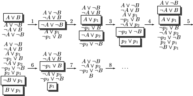
Thus, we obtain a nearly complete correspondence between search states of the explicit case analysis and the system with the binary splitting without backtracking. It is not an exact correspondence for several reasons. Firstly, simplification rules behave in a slightly different way. Secondly, splits done by splitting without backtracking often do not belong to particular branches, but are "shared" across different branches. To explain this effect, we show in Figure 2 a derivation using binary splitting and a blocking selection function which corresponds to the derivation of Figure 1. We preserve the same enumeration of inferences as in that figure. If a literal in the new signature a113 is selected, we put it in front of the clause, for example ❭ ✶ ✫ ✠ ➀ means that ❭ ✶ ✫ is selected. For simplicity, we remove subsumed clauses and pure literals.
After inference 7 of the derivation using explicit case analysis, we have a copy of the clause ❭ ❿ ✠ ❭ ➀ which was put on the right branch, after we performed a split on this clause on the left branch. In the derivation using binary splitting, the split of ❭ ❿ ✠ ❭ ➀ into ❭ ❿ ✠ ✶ ✭ and ❭ ✶ ✭ ✠ ❭ ➀ remains even when we finish working on the left branch.
4.2 Parallel extension of a selection function
Definition 4.2 (parallel extension) Let ❁ be any selection function on the clauses of the signature ♣ . The parallel extension of ❁ is a selection function ❁ ❻ on the clauses of the signature ♣ ✄ a113 defined as follows. Let ❇ be a clause of the form ❇ ❻ ✠ ➯ , where ❇ ❻ is a clause of the signature ♣ and ➯ is a clause of the signature a113 . If ❇ ❻ is not empty, then ❁ ❻ selects in ❇ ❻ ✠ ➯ exactly the same literals as ❁ selects in ❇ ❻ . When ❇ ❻ is empty, the maximal literal from ➯ is selected.
In other words, the parallel extension always makes the selection in a clause ❇ ignoring the literals of ❇ ❻ of the signature a113 .
Again, it is not difficult to prove that we indeed obtain a selection function, since all literals of the signature a113 are less than all literals of the signature ♣ . We will simply speak about a parallel selection function instead of the parallel extension of a selection function.
A parallel selection function ignores the splitting history of clause completely, and thus gives the effect of parallel search on all branches.
4.3 Subsumption resolution and splitting
One of the serious advantages of splitting without backtracking is that it can be productively combined with the simplification rule called subsumption resolution [Bachmair and Ganzinger, 2001]. Essentially, subsumption resolution is a special case of binary resolution that guarantees that the resolvent subsumes one of the parents. We say that a clause ❇ ✫ subsumes a clause ❇ ✭ if there exists a substitution ➵ such that ❇ ✫ ➵ ➸ ❇ ✭ . It is known that clauses subsumed by other clauses can be removed from the search space.
Subsumption resolution is the following inference rule on sets of clauses:
where there exists a substitution ➵ such that ❿ ✫ ➵ ❂ ❿ ✭ and ❇ ✫ ➵ ➸ ❇ ✭ . The rule is called subsumption resolution because of its resemblance to subsumption: this rule is applicable if and only if ❿ ✫ ✠ ❇ ✫ subsumes ❿ ✭ ✠ ❇ ✭ . Thus subsumption algorithms can be modified for finding pairs of clauses to which subsumption resolution is applicable.
Since subsumption resolution is a simplification rule (the clause ❭ ❿ ✭ ✠ ❇ ✭ or ❿ ✭ ✠ ❇ ✭ is replaced by a smaller clause ❇ ✭ ), it can be applied independently of the selection function or order on literals.
Subsumption resolution combined with splitting can give the following effect: literals can be moved across different branches. For example, consider two clauses ✪ ✠ ✶ and ❇ ✠
❭ ✶ such that ✪ subsumes ❇ . In explicit case analysis, these clauses would belong to two different branches, because ✪ ✠ ✶ should be on the left branch of splitting on ✶ , while ❇ ✠ ❭ ✶ on the right branch. If we use subsumption resolution, we can replace ❇ ✠ ❭ ✶ by the clause ❇ , which corresponds to moving ❇ from the right branch to the top.
The effect of subsumption resolution is even stronger when ✪ is a variant of ❇ or coincides with ❇ . Then we obtain two clauses ✪ ✠ ✶ and ✪ ✠ ❭ ✶ , which by subsumption resolution followed by subsumption will be replaced by ✪ . This has the effect of noting that ✪ belongs to two different branches, and putting it on top and can save a lot of resources compared to explicit case analysis. Splitting with backtracking would repeat inferences with ✪ on different branches.
Let us show that subsumption resolution and splitting can, in some cases, give the effect of condensing a clause. Condensing is defined in [Joyner, Jr., 1976]. A clause ❇ ❻ is said to be obtained from a clause ❇ by condensing if ❇ ❻ is a proper subset of ❇ and ❇ subsumes ❇ ❻ .
Example 4.3 Let ✪ ❈ ➼ ④ ❊ be a clause with variables in ➼ ④ and ➼ ➚ be a sequence of variables disjoint from ➼ ④ . Then ✪ ❈ ➼ ➚ ❊ is a variant of ✪ ❈ ➼ ④ ❊ . Consider the clause ✪ ❈ ➼ ④ ❊ ✠ ✪ ❈ ➼ ➚ ❊ . This clause can be condensed into ✪ ❈ ➼ ④ ❊ . Binary splitting will replace this clause by two clauses ✪ ❈ ➼ ④ ❊ ✠ ✶ and ✪ ❈ ➼ ➚ ❊ ✠ ❭ ✶ ❢ Application of subsumption resolution to these clauses yields the clause ✪ ❈ ➼ ④ ❊ which subsumes each of these clauses. Thus, binary splitting and subsumption resolution in this example give the effect of condensing.
5 Complexity of splitting with naming
To implement splitting with naming, it is required to check whether a component is a variant of another component. In this section we prove that the complexity of checking whether one clause is a variant of another one is polynomial-time equivalent to the graph isomorphism problem.
Definition 5.1 (clause variance problem) Clause variance is the following decision problem. An instance of this problem is a pair of clauses ✇ ✪ ✫ ❴ ✪ ✭ ② . The answer is "yes" if ✪ ✫ is a variant of ✪ ✭ .
Theorem 5.2 The clause variance problem is polynomialtime equivalent to the graph isomorphism problem.
The proof is given in the full version of this paper.
More generally, in practice we have to check whether a given component ✪ is a variant of a component in a set of components ✂ . In VAMPIRE we implement this many-to-one clause variance check using the code tree indexing described in [Voronkov, 1995; Riazanov and Voronkov, 2000b]. Code trees are used in the implementation of many-to-one forward subsumption, it is not hard to modify them to implement the many-to-one clause variance.
6 Experimental results
We implemented several versions splitting with backtracking in the new version of VAMPIRE [Riazanov and Voronkov, 2001]. In this section we present experimental results over 4658 nonunit clause form problems. Of these problems, 2820 problems come from the TPTP library [Sutcliffe and Suttner, 1998] and 1838 problems from the experiments in list software reuse described in [Schumann and Fischer, 1997]. Of the 4658 problems 3300 contain equality. For problems with equality, in addition to splitting without backtracking we implemented the branch rewriting rule which replaces a clause ✪ ❈ ❁ ➵ ❊ ✠ ➯ by a clause ✪ ❈ ❃ ➵ ❊ ✠ ➯ , if a clause ❁ ❂ ❃ ✠ ➯ ❻ with ➯ ❻ ➸ ➯ is present. The effect of this simplification rule is similar to the effect of simplification by unit equalities on a splitting branch in an explicit case analysis procedure. To support our viewpoint that we describe a "cheap" implementation of rewriting, we note that branch rewriting was implemented in less than 3 hours.
We present the results for problems with and without equality separately. For all problems we used the same algorithm based on the limited resource strategy [Riazanov and Voronkov, 2000a] and the same selection function. This algorithm and selection function were chosen because they experimentally proved to be superior to other algorithms and selection functions when splitting was not used. When running VAMPIRE with splitting, we used the following parameters:
- Hyper splitting with a Parallel selection function (P) vs. binary splitting with no selection.
| no | 166:11220:7227:12 | 256:6 | 280:4 | 300:1 | 359:3 | 388:3 | |
| PNR | 94:36 | 75:15 | 125:30 | 130:9 | 153:9 | 215:14241:11 | |
| NR | 71:69 | 43:6 | 121:58127:41 | 147:4 | 175:3 | ||
| PN | 95:60 | 111:50104:20180:39198:28 | |||||
| N | 98:72 | 101:52 | 115:9 | 143:8 | |||
| PR | 68:45 | 118:38144:35 | |||||
| P | 110:53130:44 | ||||||
| R | 37:8 | ||||||
| PNR NR | PN | N | PR | P | R |
| PN | 65:3 | 74:11 | 76:0 | 80:1 |
| N | 14:13 | 16:2 | 18:1 | |
| no | 19:6 | 21:5 | ||
| P | 10:7 | |||
| N | no | P |
- Naming (N) vs. no naming.
- Branch Rewriting (R) vs. no branch rewriting.
We will use combinations of the three letters P, N, R, to denote different strategies used in the experiments. For example, PR means that the Parallel version with branch Rewriting but no naming was used. We use "no" to denote the strategy that uses no splitting at all, and ➶ the strategy that uses splitting without P,R, and N, i.e. simple binary splitting with a blocking selection function.
We used a Linux-running PC with 256M RAM and a 400MHz Intel III processor. For all problems we used the time limit of 1 minute. The chosen strategy without splitting solves 3091 problems. The total number of problems solved with or without splitting is 3189. So with splitting, VAMPIRE could solve 98 problems that could not be solved without splitting. Of these 98 problems, 77 are without equality and 21 with equality. Figures 3 and 4 show the comparative behavior of various strategies depending on the settings of the parameters P, N, R on problems with and without equality, respectively. The pair ❽ ✫ ➹ ❽ ✭ in a row labelled by a strategy ✂ ✫ and the column labelled by a strategy ✂ ✭ means that there were ❽ ✫ problems solved by ✂ ✫ but not solved by ✂ ✭ and ❽ ✭ problems solved by ✂ ✭ but not solved by ✂ ✫ . For example NR (Naming + branch Rewriting) could solve 71 problems with equality not solved by PN (Parallel selection + Naming), while PN could solve 69 problems with equality not solved by NR.
The following conclusion can be derived from these results:
- On problems with equality, VAMPIRE with any version of splitting is on the average weaker than VAMPIRE without splitting, while on problems without equality it is on the average stronger.
- Each of the following settings: naming, parallel splitting, and branch rewriting improve the results, by far the strongest one is naming.
We believe that the performance of splitting without backtracking can be considerably improved, but optimized implementation, more experiments, and insights in the behavior of splitting are required.
@inproceedings{ijcai2001p85,
  title     = {Splitting Without Backtracking},
  author    = {Riazanov, Alexandre and Voronkov, Andrei},
  booktitle = {Proceedings of the Seventeenth International Joint Conference on
               Artificial Intelligence, {IJCAI-01}},
  publisher = {International Joint Conferences on Artificial Intelligence},
  editor    = {Bernhard Nebel},
  pages     = {611--616},
  year      = {2001},
  url       = {https://ijcai.org/proceedings/2001/85},
}
TY - CPAPER TI - Splitting Without Backtracking AU - Riazanov, Alexandre AU - Voronkov, Andrei T2 - Proceedings of the Seventeenth International Joint Conference on Artificial Intelligence, IJCAI-01 PB - International Joint Conferences on Artificial Intelligence PY - 2001 SP - 611 EP - 616 UR - https://ijcai.org/proceedings/2001/85 ER -Copied
Machine-readable versions of this paper, for tools and AI agents:





