Mode Estimation of Model-based Programs: Monitoring Systems with Complex Behavior

1 Introduction

Highly autonomous systems are being developed, such as NASA's Deep Space One probe (DS-1) and the X-34 Reusable launch vehicle, that involve sophisticated modelbased planning and mode-estimation capabilities to support autonomous commanding, monitoring and diagnosis. Given an observation sequence, a mode estimator, such as Livingstone [Williams and Nayak, 1996], incrementally tracks the most likely state trajectories of a system, in terms of the correct or faulty modes of every component.

A recent trend is to aggregate autonomous systems into robotic networks, for example, that create multi-spacecraft telescopes, perform coordinated Mars exploration, or perform multi vehicle search and rescue. Novel model-based methods need to be developed to monitor and coordinate these complex systems.

An example of a complex device is DS-1, which flies by an asteroid and comet using ion propulsion. DS-1's basic functions include weekly course correction (called optical navigation), thrusting along a desired trajectory, taking science readings and transferring data to earth. Each function involves a complex coordination between software and hardware. For example, optical navigation (OPNAV) works by taking pictures of three asteroids, and by using the difference between

Vineet Gupta

PurpleYogi, Inc. 201 Ravendale Drive Mountain View CA 94043 vineet@purpleyogi.com

actual and projected locations to determine the course error. OPNAV first shuts down the Ion engine and prepares its camera concurrently. It then uses the thrusters to turn to each of three asteroids, uses the camera to take a picture of each, and stores each picture on disk. The three images are then read, processed and a course correction is computed. One of the more subtle failures that OPNAV may experience is a corrupted camera image. The camera generates a faulty image, which is stored on disk. At some later time the image is read, processed, and only then is the failure detected. A monitoring system must be able to estimate this event sequence based on the delayed symptom.

Diagnosing the OPNAV failure requires tracking a trajectory that reflects the above description. Identifying this trajectory goes well beyond Livingstone's abilities. Livingstone, like most diagnostic systems, focuses on monitoring and diagnosing networks whose components, such as valves and bus controllers, have simple behaviors. However, the above trajectory spends most of its time wending its way through software functions. DS-1 is an instance of modern embedded systems whose components involve a mix of hardware, computation and software. Robotic networks extend this trend to component behaviors that are particularly sophisticated.

This paper addresses the challenge of modeling and monitoring systems composed of these complex components. We introduce a unified language that can express a rich set of mixed hardware and software behaviors (the Reactive Modelbased Programming Language [RMPL]). RMPL merges constructs from synchronous programming languages, qualitative modeling, Markov models and constraint programming. Synchronous, embedded programming offers a class of languages developed for writing control programs for reactive systems [Benveniste and Berry, 1991; Saraswat et al., 1996] - logical concurrency, preemption and executable specifications. Markov models and constraint-based modeling[Williams and Nayak, 1996] offer rich languages for describing uncertainty and continuous processes at the qualitative level.

Given an RMPL model, we frame the problem of monitoring robotic components as a variant of belief update on a hidden Markov model (HMM), where the HMM of the system is described in RMPL. A key issue is the potentially enormous state space of RMPL models. We address this by introducing a hierachical, constraint-based encoding of an HMM, called a probabilistic, hierarchical, constraint automata (PHCA). Next we show how RMPL models can be compiled to equivalent PHCAs. Finally, we demonstrate one approach in which RMPL belief update can be performed by operating directly on the compact PHCA encoding.

2 HMMs and Belief Update

The theory of HMMs offers a versatile tool for framing hidden state interpretation problems, including data transmission, speech and handwriting recognition, and genome sequencing. This section reviews HMMs and state estimation through belief update.

AnHMM is described by a tuple a0 ✁ ✄ ✆ ✄ ✟ ✡ ✄ ✟ ✍ ✄ ✟ ✆ ✑ . ✁ and ✆ denote finite sets of feasible states ✒ ✓ and observations ✕ ✓ . The initial state function, ✟ ✡ ✖ ✒ ✓ ✗ ✙ ✛ ✢ , denotes the probability that ✒ ✓ is the initial state. The state transition function, ✟ ✍ ✖ ✒ ✓ ✗ ✤ ✛ ✦★ ✒ ✓ ✗ ✤ ✪ ✫ ✛ ✢ , denotes the conditional probability that ✒ ✓ ✗ ✤ ✪ ✫ ✛ is the next state, given current state ✒ ✓ ✗ ✤ ✛ at time ✰ . The observation function, ✟ ✆ ✖ ✒ ✓ ✗ ✤ ✛ ✦★ ✕ ✓ ✗ ✤ ✛ ✢ denotes the conditional probability that ✕ ✓ ✗ ✤ ✛ is observed, given state ✒ ✓ ✗ ✤ ✛ .

Belief update incrementally computes the current belief state, that is, the likelihood that the system is in any state ✒ ✓ , conditioned on each control action performed and observation received, respectively:

✱ ✗ ✲ ✤ ✪ ✫ ✛ ✖ ✒ ✓ ✢ ✶ P ✖ ✒ ✓ ✗ ✤ ✪ ✫ ✛ ✸ ✕ ✗ ✙ ✛ ✺ ✻ ✄ ✼ ✼ ✼ ✄ ✕ ✗ ✤ ✛ ✺ ✿ ✄ ❀ ✗ ✙ ✛ ✺ ✻ ✼ ✼ ✼ ❀ ✗ ✤ ✛ ✺ ✿ ✢ ✱ ✗ ✤ ✪ ✫ ✲ ✛ ✖ ✒ ✓ ✢ ✶ P ✖ ✒ ✓ ✗ ✤ ✪ ✫ ✛ ✸ ✕ ✗ ✙ ✛ ✺ ✻ ✄ ✼ ✼ ✼ ✄ ✕ ✗ ✤ ✪ ✫ ✛ ✺ ✿ ✪ ✫ ✄ ❀ ✗ ✙ ✛ ✺ ✻ ✼ ✼ ✼ ❀ ✗ ✤ ✛ ✺ ✿ ✢

Exploiting the Markov property, the belief state at time ✰ ❁ ❃ is computed from the belief state and control actions at time ✰ and observations at ✰ ❁ ❃ using the standard equations. For simplicity, control actions are made implicit within ✟ ✍ :

✱ ✗ ✲ ✤ ✪ ✫ ✛ ✖ ✒ ✓ ✢ ❇ ❈ ❉ ❊ ❋ ✫ ✱ ✗ ✤ ✲ ✛ ✖ ✒ ❊ ✢ ✟ ✍ ✖ ✒ ❊ ✦★ ✒ ✓ ✢ ✱ ✗ ✤ ✪ ✫ ✲ ✛ ✖ ✒ ✓ ✢ ❇ ✱ ✗ ✲ ✤ ✪ ✫ ✛ ✖ ✒ ✓ ✢ ✟ ✆ ✖ ✒ ✓ ✦★ ✕ ■ ✢ ❑ ❈ ❊ ❋ ✫ ✱ ✗ ✲ ✤ ✪ ✫ ✛ ✖ ✒ ❊ ✢ ✟ ✆ ✖ ✒ ❊ ✦★ ✕ ■ ✢

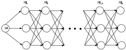
The space of possible trajectories of an HMM can be visualized using a Trellis diagram, which enumerates all possible states at each time step and all transitions between states at adjacent times. Belief update associates a probability to each state in the graph.

3 Design Desiderata for RMPL

Returning to our example, OPNAV is best expressed at toplevel as a program:

OpNav() :: ▲ TurnCameraOn, if EngineOn thennext SwitchEngineStandBy, do when EngineStandby ▼ CameraOn donext ▲ TakePicture(1); TakePicture(2); TakePicture(3); ▲ TurnCameraOff, ComputeCorrection() ◆ ◆ watching PictureError ❖ OpticalNavError, when OpticalNavError donext OpNav(), when PictureError donext OpNavFailed ◆

In this program comma delimits parallel processes and semicolon delimits sequential processes.

OPNAV highlights four key design features for RMPL. First, the program exploits full concurrency, by intermingling sequential and parallel threads of execution. For example, the camera is turned on and the engine is turned off in parallel, while pictures are taken serially. Second, it involves conditional execution, such as switching to standby if the engine is on. Third, it involves iteration; for example, "when Engine Standby ✼ ✼ ✼ donext ✼ ✼ ✼ " says to iteratively test to see if the engine is in standby and if so proceed. Fourth, the program involves preemption; for example, "do ✼ ✼ ✼ watching " says to perfom a task, but to interrupt it as soon as the watch condition is satisfied. Subroutines used by OpNav, such as TakePicture, exploit similar features.

OpNav also relies on hardware behaviors, such as:

Camera :: always ▲ choose ▲ ▲ if CameraOn then ▲ if TurnCameraOff thennext MicasOff elsenext CameraOn, if CameraTakePicture thennext CameraDone ◆ , if CameraOff then if TurnCameraOn thennext CameraOn elsenext CameraOff, if CameraFail then if MicasReset thennext CameraOff elsenext CameraFail ◆ with0.99, next CameraFail with 0.01 ◆ ◆

OpNav's tight interaction with hardware makes the overall process stochastic. We add probabilistic execution to our design features to model failures and uncertain outcomes. We add constraints to represent co-temporal interactions between state variables. Summarizing, the key design features of RMPL are full concurrency, conditional execution, iteration, preemption, probabilistic choice, and co-temporal constraint.

4 RMPL: Primitive Combinators

Our preferred approach to developing RMPL is to introduce a minimum set of primitives for constructing programs, where each primitive is driven by one of the six design features of the preceding section. To make the language usable we define on top of these primitives a variety of program combinators, such as those used in the optical navigation example. In the following we use lower case letters, like a0 , to denote constraints, and upper case letters, like ✁ and ✂ , to denote well-formed RMPL expressions. The term "theory" refers to the set of all constraints that hold at some time point.

• a0 . This programasserts that constraint a0 is true at the initial instant of time.
• if a0 thennext ✁ . This programstarts behaving like ✁ in the next instant if the current theory entails a0 . This is the basic conditional branch construct.

unless a0 thennext ✁ . This program executes ✁ in the next instant if the current theory does not entail c. This is the basic construct for building preemption constructs. It allows A to proceed as long as some condition is unknown, but stops when the condition is determined.

• ✁ ✄ ✂ . This program concurrently executes A and B, and is the basic construct for forking processes.

always ✁ . This program starts a new copy of ✁ at each instant of time, for all time. This is the only iteration construct needed, since finite iterations can be achieved by using if or unless to terminate an always .

choose ✖ ✁ with ☎ ✄ ✂ with ✆ ✢ . This is the basic combinator for expressing probabilistic knowledge. It reduces to program ✁ with probability ☎ , to program ✂ with probability ✆ , and so on. For simplicity we would like to ensure that constraints in the current theory do not depend upon probabilistic choices made in the current state. We achieve this by restricting all constraints asserted within ✁ and ✂ to be within the scope of an if ✼ ✼ ✼ next or unless ✼ ✼ ✼ next.

These six primitive combinators cover the six design features. They have been used to implement a rich set of derived combinators [anonymous] including those in the OpNav example, and most from the Esterel language [Berry and Gonthier, 1992]. The derived operators for OpNav, built from these primitives, is given in Appendix A.

5 Hierarchical, Constraint Automata

To estimate RMPL state trajectories we would like to map the six RMPL combinators to HMMs and then perform belief update. However, while HMMs offer a natural way of thinking about reactive systems, as a direct encoding they are notoriously intractable. One of our key contributions is a representation, called Probabilistic, Hierarchical, Constraint Automata (PHCA) that compactly encodes HMMs describing RMPL models.

PHCA extend HMMs by introducing four essential attributes. First, the HMM is factored into a set of concurrently operating automata. Second, each state is labeled with a constraint that holds whenever the automaton marks that state. This allows an efficient encoding of co-temporal processes, such as fluid flows. Third, automata are arranged in a hierarchy - the state of an automaton may itself be an automaton, which is invoked when marked by its parent. This enables the initiation and termination of more complex concurrent and sequential behaviors. Finally, each transition may have multiple targets, allowing an automaton to be in several states simultaneously. This enables a compact representation for recursive behaviors like "always" and "do until".

The first two attributes are prevalent in areas like digital systems and qualitative modeling. The third and fourth form the basis for embedded reactive languages like Esterel[Berry and Gonthier, 1992], Lustre[Halbwachs et al., 1991], Signal[Guernic et al., 1991] and State Charts[Harel, 1987]. Together they allow complex systems to be modeled that involve software, digital hardware and continuous processes.

We develop PHCAs by first introducing a deterministic equivalent, and then extending to Markov models. We describe a deterministic, hierarchical, constraint automaton (HCA) as a tuple a0 ✁ ✄ ✡ ✄ ✝ ✄ ✆ ✄ ✟ ✡ ✄ ✍ ✡ ✑ , where:

• ☞ ✁ is a set of states, partitioned into primitive states ✁ ✌ and composite states ✁ ✎ . Each composite state denotes a hierarchical, constraint automaton.
• ☞ ✡ ✑ ✁ is the set of start states (also called the initial marking).
• ☞ ✝ is a set of variables with each ✓ ✓ ✔ ✝ ranging over a finite domain ✗ ✖ ✓ ✓ ✢ . ✟ ✖ ✝ ✢ denotes the set of all finite domain constraints over ✝ .
• ☞ ✆ ✑ ✝ is the set of observable variables.
• ☞ ✟ ✡ ✘ ✁ ✌ ★ ✟ ✖ ✝ ✢ , associates with each primitive state ✒ ✓ a finite domain constraint ✟ ✡ ✚ ✒ ✓ ✛ that holds whenever ✒ ✓ is marked.
• ☞ ✍ ✡ ✘ ✁ ✌ ✣ ✟ ✖ ✝ ✢ ★ ✥ ✁ associates with each primitive state ✒ ✓ a transition function ✍ ✡ ✚ ✒ ✓ ✛ . Each ✍ ✡ ✚ ✒ ✓ ✛ ✘ ✟ ✖ ✝ ✢ ★ ✥ ✁ , specifies a set of states to be marked at time ✰ ❁ ❃ , given assignments to ✝ at time ✰ .

At any instant ✰ the "state" of an HCA is the set of marked states ★ ✓ ✗ ✤ ✛ ✩ ✁ , called a marking. ✫ denotes the set of possible markings, where ✫ ❇ ✥ ✁ .

Consider the combinator always ✁ , which maps to:

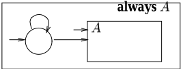
This automaton starts a new copy of ✁ at each time instant. The states ✁ of the automaton consist of primitive state ✒ ❈ ✬ ✮ , drawn to the left as a circle, and composite state ✁ , drawn to the right as a rectangle. The start states ✡ are ✒ ❈ ✬ ✮ and ✁ , as is indicated by two short arrows.

A PHCA models physical processes with changing interactions by enabling and disabling constraints within a constraint store (e.g., opening a valve causes fuel to flow to an engine). RMPL currently supports propositional state logic as its constraint system. In state logic each proposition is an assignment ✓ ✓ ❇ ✰ ✓ ❊ , where variable ✓ ✓ ranges over a finite domain ✗ ✚ ✓ ✓ ✛ . Constraints ✟ ✡ are indicated by lower case letters, such as a0 , written in the middle of a primitive state. If no constraint is indicated, the state's constraint is implicitly True. In the above example ✒ ❈ ✬ ✮ implicitly has constraint True; other constraints may be hidden within ✁ .

Transitions between successive states are conditioned on constraints entailed by the store (e.g., the presence or absence of acceleration). This allows us to model indirect control and indirect effects. For each primitive state ✒ we represent the transition function ✍ ✡ ✚ ✒ ✛ as a set of (transition) pairs ✚ a0 ✓ ✄ ✒ ✓ ✛ , where ✒ ✓ ✔ ✁ , and a0 ✓ is a set of labels of the form ✸ ❇ a0 or ✂ ✸ ❇ a0 , for some a0 ✔ ✟ ✖ ✝ ✢ . This corresponds to the traditional representation of transitions, as labeled arcs in a graph, where ✒ and ✒ ✓ are the source and destination of an arc with label a0 ✓ . For convenience, in our diagrams we use a0 to denote the label ✸ ❇ a0 , and a0 to denote the label ✂ ✸ ❇ a0 . If no label is indicated, it is implicitly ✸ ❇ True. The above example has two transitions, both with labels that are implicitly ✸ ❇ True.

Our HCA encoding has three key properties that distinguish it from the hierarchical automata employed by reactive embedded languages[Benveniste and Berry, 1991; Harel, 1987]. First, multiple transitions may be simultaneously traversed. This allows an extremely compact encoding of the state of the automaton as a set of markings. Second, transitions are conditioned on what can be deduced, not just what is explicitly assigned. This provides a simple but general mechanism for incorporating constraint systems that reason about indirect effects. Third, transitions are enabled based on lack of information. This allows default executions to be pursued in the absence of better information, enabling advanced preemption constructs.

6 Executing HCA

To execute an automata A, we first initialize it using ★ ✄ ✚ ✡ ✚ ✁ ✛ ✛ , which marks the start states of all its subautomata, and then step it using ✆ ✰ ✝ ☎ ✚ ✁ ✛ , which maps its current marking to a next marking. 1

A trajectory of automaton ✁ is a sequence of markings ★ ✓ ✗ ✙ ✛ ✄ ★ ❊ ✗ ✫ ✛ ✄ ✼ ✼ ✼ such that ★ ✓ ✗ ✙ ✛ is the initial marking ★ ✄ ✚ ✡ ✛ , and for each a0 ✟ ✡ , ★ ✓ ✗ ☞ ✪ ✫ ✛ ❇ ✆ ✰ ✝ ☎ ✚ ✁ ✄ ★ ❊ ✗ ☞ ✛ ✛ .

Given a set of automata ★ to be initialized, ★ ✄ ✚ ★ ✛ creates a full marking, by recursively marking the start states of ★ and all their descendants:

For example, applying ★ ✄ to automata always ✁ , returns the set consisting of always ✁ , ✒ ❈ ✬ ✮ , ✁ and any start states contained within ✁ .

✆ ✰ ✝ ☎ transitions an automaton A from one full marking to the next:

✆ ✰ ✝ ☎ ✚ ✁ ✄ ★ ✓ ✗ ✤ ✛ ✛ ★ ★ ❊ ✗ ✤ ✪ ✫ ✛ :: ❃ ✼ ✖ ❃ ✘ ❇ ✒ ✒ ✔ ★ ✓ ✗ ✤ ✛ ✸ ✒ is primitive✔ ✥ ✼ ✘ ✘ ❇ ✙ ✛ ✜ ✣ ✫ ✟ ✡ ✚ ✒ ✛ ✥ ✼ ✖ ✥ ✘ ❇ ✦ ✛ ✜ ✣ ✫ ✍ ✡ ✚ ✒ ✄ ✘ ✛ ✩ ✼ return ★ ✄ ✚ ✖ ✥ ✛

1 Execution "completes" when no marks remain, since the empty marking is a fixed point.

✆ ✰ ✝ ☎ involves identifying the marked primitive states (Step 1), collecting the constraints of these marked states into a constraint store (Step 2), identifying the transitions of marked states that are enabled by the store and the resulting states reached (Step 3), and, initializing any automata reached by this transition (Step 4). The result is a full marking for the next time step.

To transition in step 3, let ✚ a0 ✓ ✄ ✒ ✓ ✛ ✔ ✍ ✡ ✚ ✒ ✛ be any transition pair of a currently marked primitive state ✒ . Then ✒ ✓ is marked in the next instant if a0 ✓ is entailed by the current constraint store, ✘ (computed in step 2). A label a0 ✓ is said to be entailed by ✘ , written ✘ ✸ ❇ a0 ✓ , if ✫ ✸ ❇ a0 ✔ a0 ✓ ✼ ✘ ✸ ❇ a0 , and for each ✂ ✸ ❇ a0 ✔ a0 ✓ ✼ ✘ ✂ ✸ ❇ a0 . 2

Applying ✆ ✰ ✝ ☎ to the initial marking of always ✁ causes ✒ ❈ ✬ ✮ to transition to ✁ and back to ✒ ❈ ✬ ✮ , and for ✁ to transition internally. The new mark on ✁ invokes a second copy of ✁ , by marking ✁ ✭ ✒ start states. More generally, ✒ ❈ ✬ ✮ is responsible for initiating A during every time step after the first. A transition back to itself ensures that ✒ ❈ ✬ ✮ is always marked. The transition to ✁ puts a newmark on ✁ at every next step, each time invoking a virtual copy of ✁ . The ability of an automaton to have multiple states marked simultaneously is key to the compactness of this novel encoding, by avoiding the need for explicit copies of A.

7 A Simple Example

As an example consider the RMPL expression:

This expression roughly maps to:

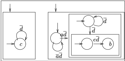
The automaton has two start states, both of which are composite. Every transition is labeled ✂ ✸ ❇ ✱ , hence all transitions are disabled and the automaton is preempted whenever d becomes true. The first state has one primitive state, which asserts the constraint a0 . If ✱ does not hold, then it goes back to itself - thus it repeatedly asserts a0 until ✱ becomes true. The second automaton has a primitive start state. Once again, at anytime if ✱ becomes true, the entire automaton will immediately terminate. Otherwise it waits until ✯ becomes true, and then goes to its second state, which is composite. This automaton has one start state, which it repeats at every time instant until ✱ holds. In addition, it starts another automaton, which checks if ✝ holds, and if true generates ✰ in the next

2 Formally, ✲ ✳ ✴ ✶ ✸ ✺ ✼ ✾ ▲ ✶ ❀ ❂ ✴ ❅ ❀ ✸ ✶ ❀ ✼ ❈ ✲ ✳ ✴ ✶ ✼ ✸ ✺ ❂ ✾ ❅ ❀ ◆ .

state. Thus, the behavior of the overall automaton is as follows: it starts asserting a0 at every time instant. If ✯ becomes true, then at every instant thereafter it checks if ✝ is true, and asserts ✰ in the succeeding instant. Throughout it watches for ✱ to become true, and if so halts.

8 Probabilistic HCA

We extend HCA to Markov processes by replacing the single initial marking and transition function of HCA with a probability distribution over possible initial markings and transition functions. We describe a probabilistic, hierarchical, constraint automata by a tuple a0 ✁ ✄ ✟ ✡ ✄ ✝ ✄ ✆ ✄ ✟ ✡ ✄ ✟ ✍ ✡ ✑ , where:

• ☞ ✁ , ✝ , ✆ and ✟ ✡ are the same as for HCA.
• ☞ ✟ ✡ ✚ ★ ✓ ✛ denotes the probability that ★ ✓ ✑ ✁ is the initial marking.
• ☞ ✟ ✍ ✡ ✚ ✒ ✓ ✛ , for each ✒ ✓ ✔ ✁ ✌ , denotes a distribution over possible transition functions ✍ ✡ ❊ ✚ ✒ ✓ ✛ ✘ ✟ ✖ ✝ ✢ ★ ✥ ✁ .

The transition function ✟ ✍ ✡ ✚ ✒ ✓ ✛ is encoded as an AND/OR tree. We present an example at the end of the next section, when describing the choose combinator.

PHCA execution is similar to HCA execution, except that ★ ✄ probabilistically selects an initial marking, and ✆ ✰ ✝ ☎ probabilistically selects one of the transition functions in ✟ ✍ ✡ for each marked primitive state. The probability of a marking ★ ✓ ✗ ✤ ✛ is computed by the standard belief update equations given in Section 2. This involves computing ✟ ✍ and ✟ ✆ .

To calculate transition function ✟ ✍ for marking ★ ✓ recall that a transition ✍ is composed of a set of primitive transitions, one for each marked primitive state ✒ ✓ , and that the PHCA specifies the transition probability for each primitive state through ✟ ✍ ✡ ✚ ✒ ✓ ✛ . We make the key assumption that primitive transition probabilities are conditionally independent, given the current marking. This is analogous to the failure independence assumptions made by GDE[de Kleer and Williams, 1987] and Livingstone[Williams and Nayak, 1996], and is a reasonable assumption for most engineered systems. Hence, the composite transition probability between two markings is computed as the product of the transition probabilities from each primitive state in the first marking to a state in the second marking.

We calculate the observation function ✟ ✆ for marking ★ ✓ from the model, similar to GDE[de Kleer and Williams, 1987]. Given the constraint store ✘ for ★ ✓ from step 2 of ✆ ✰ ✝ ☎ , we test if each observation in ✕ ✓ is entailed or refuted, giving it probability 1 or 0, respectively. If no prediction is made, then an a priori distribution on observables is assumed (e.g., a uniformdistribution of ❃ a0 ✂ for ✂ possible values).

This completes PHCA belief update. Our remaining tasks are to compile RMPL to PHCA, and to implement belief update efficiently.

9 Mapping RMPL to PHCA

Each RMPL primitive maps to a PHCA as defined below. RMPL sub-expressions, denoted by upper case letters, are recursively mapped to equivalent PHCA.

• a0 . Asserts constraint a0 at the initial instant of time:

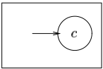
The start state has no exit transitions, so after this automaton asserts a0 in the first time instant it terminates.

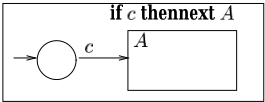
if a0 thennext ✁ . Behaves like ✁ in the next instant if the current theory entails a0 . Given the automaton for ✁ , we add a new start state, and a transition from this state to ✁ when a0 is entailed:

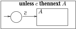
unless a0 thennext ✁ . Executes ✁ in the next instant if the current theory does not entail c. This mapping is analogous to if a0 thennext ✁ . It is the only construct that introduces condition ✂ ✸ ❇ a0 . This introduces non-monotonicity; however, since these non-monotonic conditions hold only in the next instant, the logic is stratified and monotonic in each state. This avoids the kinds of causal paradoxes possible in languages like Esterel[Berry and Gonthier, 1992].

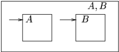
always ✁ . Starts a new copy of ✁ at each time instant, as described in Section 5.

choose ✖ ✁ with ☎ ✄ ✂ with ✆ ✢ . Reduces to ✁ with probability ☎ , to ✂ with probability ✆ , and so on. Recall that we required that all constraints asserted within ✁ and ✂ must be within the scope of a next. This ensures that probabilities are associated only with transitions. The corresponding automaton is encoded with a single probabilistic start transition, which allows us to choose between ✁ and ✂ . This is the only combinator that introduces probabilistic transitions.

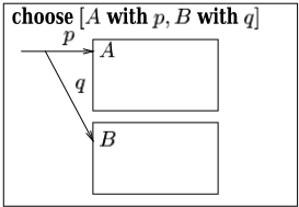
Encoding probabilistic choice requires special attention due to the use of nested choose expressions. We encode the transition function ✍ ✡ ✚ ✒ ✓ ✛ as a probabilistic AND-OR tree (below, left), enabling a simple transformation from nested choose expressions to a PHCA.

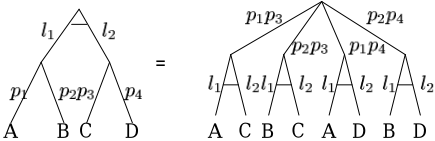
In this tree each leaf is labeled with a set of one or more target states in ✁ , which the automaton transitions to in the next time step. The branches ✯ ✓ ★ ✰ ✓ ❊ of a probabilistic OR node ✯ ✓ represent a distribution over a disjoint set of alternatives, and are labeled with conditional probabilities P ✖ ✰ ✓ ❊ ✸ ✯ ✓ ✢ . These are ☎ ✫ ✼ ✼ ✼ ☎ ☎ in the left tree. The probabilities of branches emanating from each OR node ✯ ✓ sum to unity.

The branches of a deterministic AND node represent an inclusive set of choices. The node is indicated by a horizontal bar through its branches. Each branch is labeled by a set of conditions a0 ✓ ❊ , as defined for HCA. These are a0 ✫ and a0 a0 in the left tree. During a transition, every branch in an AND node is taken that has its label satisfied by the current state (i.e., P ✖ ✰ ✓ ❊ ✸ ✯ ✓ ✄ a0 ✓ ❊ ✢ ❇ ❃ ).

Tomap this tree to ✍ ✡ ✚ ✒ ✓ ✛ , eachAND-OR tree is compiled to a two level tree (shown above, right), with the root node being a probabilistic OR, and its children being deterministic ANDs. Compilation is performed using distributivity, shown by the figure, and commutativity. Commutativity allows adjacent AND nodes to be merged, by taking conjunctions of labels, and adjacent OR nodes to be merged, by taking products of probabilities. This two level tree is a direct encoding of ✍ ✡ ✚ ✒ ✓ ✛ . Each AND node represents one of the transition functions ✍ ✡ ❊ ✚ ✒ ✓ ✛ , while the probability on the OR branch, terminating on this AND node, denotes ✟ ✚ ✍ ✡ ❊ ✚ ✒ ✓ ✛ ✛ .

10 PHCAEstimation as Beam Search

We demonstrate PHCA belief update with a simple implementation of mode estimation, called RMPL-ME, that follows Livingstone[Williams and Nayak, 1996]. Livingstone tracks the most likely trajectories through the Trellis diagram by using beam search, which expands only the highest probability transitions at each step. To implement this we first modify ✆ ✰ ✝ ☎ , defined for HCA, to compute the likely states of ✱ ✗ ✲ ✤ ✪ ✫ ✛ ✖ ★ ✓ ✢ . This new version, Step ✡ , returns a set of markings, each with its own probability.

✆ ✰ ✝ ☎ ✡ ✚ ✁ ✄ ★ ✓ ✗ ✤ ✛ ✛ ★ ★ ❊ ✗ ✤ ✪ ✫ ✛ ::

• ❃ ✼ ✖ ❃ ✘ ❇ ✒ ✒ ✔ ★ ✓ ✗ ✤ ✛ ✸ ✒ is primitive✔
• ✥ ✼ ✘ ✘ ❇ ✙ ✛ ✜ ✣ ✫ ✟ ✡ ✚ ✒ ✛
• ✥ ✯ ✼ ✖ ✥ ✯ ✘ ❇ ✟ ✛ ✜ ✣ ✫ ✍ ✡ ✚ ✒ ✄ ✘ ✛
• ✥ ✰ ✼ ✖ ✥ ✰ ✘ ❇ ✒ ✚ ★ ✄ ✚ ✦ ❈ ✓ ❋ ✫ ✒ ✒ ✓ ✔ ✛ ✄ ✟ ❈ ✓ ❋ ✫ ☎ ✓ ✛ ✸ a0 ✚ ✒ ✫ ✄ ☎ ✫ ✛ ✄ ✼ ✼ ✼ ✄ ✚ ✒ ❈ ✄ ☎ ❈ ✛ ✑ ✔ ✖ ✥ ✯ ✔
• ✥ a0 ✼ ★ ❊ ✗ ✤ ✪ ✫ ✛ ✘ ❇ ✒ ✚ ✆ ✄ ❑ ✗ ✠ ☛ ✌ ✛ ✜ ✣ a0 ✌ ☎ ✛ ✸ ✚ ✆ ✄ ☎ ✛ ✔ ✖ ✥ ✰ ✔
• ✩ ✼ return ★ ❊ ✗ ✤ ✪ ✫ ✛

Step 3a builds the sets of possible primitive transitions. Step 3b computes for each set the combined next state marking and transition probability. Step 3c sums the probabilities of all composite transitions with the same target. Step 4 returns this approximate belief state. In Steps 3a and b, we enumerate transition sets in decreasing order of likelihood until most of the probability density space is covered (e.g., ✎ ✏ ✒ ). Best first enumeration is performed using our OPSAT system, generalized from [Williams and Nayak, 1996]. OPSAT finds the leading solutions to the problem " ✯ ✓ ✔ ✖ ✘ ✚ ✜ ✚ ✣ ✛ subject to ✘ ✚ ✣ ✛ ," where ✣ is a state vector, ✘ ✚ ✣ ✛ is a set of propositional state constraints, and ✜ ✚ ✣ ✛ is an additive, multi-attribute utility function. OPSAT tests a leading candidate for consistency against ✘ ✚ ✣ ✛ . If it proves inconsistent, OPSAT summarizes the inconsistency (called a conflict) and uses the summary to jump over leading candidates that are similarly inconsistent.

After computing the leading states of ✱ ✗ ✲ ✤ ✪ ✫ ✛ ✖ ★ ✓ ✢ , RMPLME computes ✟ ✆ ✖ ★ ✓ ✗ ✤ ✛ ✦★ ✕ ✓ ✗ ✤ ✛ ✢ using the constraint store extracted in step 2, and uses these results to compute the final result ✱ ✗ ✤ ✪ ✫ ✲ ✛ ✖ ★ ✓ ✢ , from the standard equation.

11 Implementation and Discussion

Implementations of the RMPL compiler, RMPL-ME and OPSAT are written in Common Lisp. The full RMPL language is an object-oriented language, in the style of Java, that supports all primitive combinators (Section 4) and a variety of defined combinators. The RMPL compiler outputs PHCA as its object code. RMPL-ME uses the compiled PHCAs to perform online incremental belief update, as outlined above. To support real-time embedded applications, RMPL-ME and OPSAT are being rewritten in C and C++.

The DS1 OpNav example provides a simple demonstration of RMP-ME. In addition RMPL-ME is being developed in two mission contexts. First, the C prototype is being demonstrated on the MIT Spheres formation flying testbed, a "robotic network" of three, soccer ball sized spacecraft that have flown on the KC-135. RMPL models are also being developed for the John Hopkins APL NEAR (Near Earth Asteroid Rendezous) mission.

Beam search is among the simplest of estimation approaches. It avoids an exponential blow up in the space of trajectories explored and avoids explicitly generating the Trellis diagram, but sacrifices completeness. Consequently it will miss a diagnosis if the beginning of its trajectory is sufficiently unlikely that it is clipped by beam search. A range of solutions to this problem exist, including an approach, due to [Hamscher and Davis, 1984], that uses a temporal constraint graph analogous to planning graphs. This encoding coupled with state abstraction methods has recently been incorporated into Livingstone [Kurien and Nayak, 2000], with attractive performance results. Another area of research is the incorporation of metric time. [Largouet and Cordier, 2000] introduces an intriguing approach based on model-checking algorithms for timed automata. Finally, [Malik and Struss, 1997] explores the discriminatory power of transitions vs state constraints in a consistency-based framework.

Acknowledgments

We would like to thank Michael Hofbaur, Howard Shrobe, Randall Davis and the anonymous reviewers for their invaluable comments. This research is supported in part by the DARPA MOBIES program under contract F33615-00-C1702 and by NASA CSOC contract G998747B17.

A RMPL Defined Operators

To express complex behaviors in RMPL, we use the six RMPL primitives to define a rich set of constructs common to embedded languages, such as recursion, conditional execution, next, sequence, iteration and preemption. This section includes a representative sample of RMPL's derived constructs, used to support the DS1 opnav example.

Recursion and procedure definitions. A recursive declaration is of the form a0 ✘ ✘ ✁ ✖ a0 ✢ , where ✁ may contain occurrences of procedure name a0 . We implement this declaration with always if ☎ then ✁ ✖ ☎ a0 a0 ✢ . At each time tick the expression looks to see if p is asserted (corresponding to p being invoked), and if so starts A. This method allows us to do parameterless recursion. Recursion with parameters is only guaranteed to be compilable into finite state automata if the recursion parameters have finite domains.

• next ✁ . This is simply if ✰ ✓ ✂ ✝ thennext ✁ . We can also define if a0 thennext ✁ ☎ ✆ ✞ ☎ ✡ ☎ ✣ ✌ ✂ as if a0 thennext ✁ ✄ unless a0 thennext ✂ .
• A; B. This is the sequential composition of ✁ and ✂ . It performs ✁ until ✁ is finished. Then it starts B. It can be written in terms of the preceding constructs by detecting the termination of ✁ by a proposition, and using that to trigger ✂ . RMPL detects the termination of ✁ by a case analysis of the structure of ✁ . [Fromherz et al., 1997] for details). For efficiency, the RMPL compiler implements A; B directly, rather than translating to basic combinators.
• do ✁ while a0 . Executes ✁ , but if a0 is not true in a state, then ✁ is terminated immediately. This combinator can be derived from the preceding combinators as follows:
• do ✎ while ✏ ✾ ✏ ✒ ✎
• do ✴ if ✎ thennext ✕ ✼ while ✏ ✾ if ✏ ▼ ✎ thennext do ✕ while ✏
• do ✴ ✕ ✸ ✗ ✼ while ✏ ✾ do ✕ while ✏ ✸ do ✗ while ✏ do ✴ always ✕ ✼ while ✏ ✾ ✙ ✸ always if ✴ ✙ ▼ ✏ ✼ then ✴ do ✕ while ✏ ✸ next ✙ ✼
• do ✴ unless ✎ thennext ✕ ✼ while ✏ ✾ if ✏ then unless ✎ thennext ✴ do ✕ while ✏ ✼
• do ✴ choose ✚ ✕ with ✛ ✸ ✗ with ✢ ✣ ✼ while ✏ ✾ choose ✴ do ✕ while ✏ with✛ ✸ do ✗ while ✏ with✢ ✼

For efficiency, RMPL derives the automaton for do ✁ while a0 from the automaton for A by adding the label ✸ ❇ a0 to all transitions in ✁ , and in addition, replacing all the propositional formulas ✥ in the states by a0 ★ ✥ . Thus if a0 is not entailed by constraints outside of A, no transition or constraint in this automaton will be enabled.

do ✁ watching a0 . This is a weak preemption operator. It executes ✁ , but if a0 becomes true in any time instant, it terminates execution of ✁ in the next instant. The automaton for this is derived from the automaton for ✁ by adding the label ✂ ✸ ❇ a0 on all transitions in ✁ .

when a0 donext ✁ . This starts ✁ at the instant after the first one in which a0 becomes true. It is a temporally extended version of if a0 thennext ✁ . and is defined as:

when a0 donext ✁ ❇ always if ✚ ✯ ✦ a0 ✛ thennext ✁ ✄ do always ✯ watching a0